library(CMTFtoolbox)
library(dplyr)
#>
#> Attaching package: 'dplyr'
#> The following objects are masked from 'package:stats':
#>
#>     filter, lag
#> The following objects are masked from 'package:base':
#>
#>     intersect, setdiff, setequal, union
library(ggplot2)
library(ggpubr)
library(rTensor)

set.seed(123)
simTensorMatrixData = function(I=108, J=100, K=10, L=100, numComponents=2){

  A = array(rnorm(I*numComponents), c(I, numComponents))  # shared subject mode
  B = array(rnorm(J*numComponents), c(J, numComponents))  # distinct feature mode of X1
  C = array(rnorm(K*numComponents), c(K, numComponents))  # distinct condition mode of X1
  D = array(rnorm(L*numComponents), c(L, numComponents))  # distinct feature mode of X2

  df1 = reinflateTensor(A, B, C)
  df2 = reinflateMatrix(A, D)
  datasets = list(df1, df2)
  modes = list(c(1,2,3), c(1,4))
  Z = setupCMTFdata(datasets, modes, normalize=TRUE)

  return(list("Z"=Z, "A"=A, "B"=B, "C"=C, "D"=D))
}

simTwoTensorData = function(I=108, J=100, K=10, L=100, M=10, numComponents=2){

  A = array(rnorm(I*numComponents), c(I, numComponents))  # shared subject mode
  B = array(rnorm(J*numComponents), c(J, numComponents))  # distinct feature mode of X1
  C = array(rnorm(K*numComponents), c(K, numComponents))  # distinct condition mode of X1
  D = array(rnorm(L*numComponents), c(L, numComponents))  # distinct feature mode of X2
  E = array(rnorm(M*numComponents), c(M, numComponents))  # distinct condition mode of X2

  df1 = reinflateTensor(A, B, C)
  df2 = reinflateTensor(A, D, E)
  datasets = list(df1, df2)
  modes = list(c(1,2,3), c(1,4,5))
  Z = setupCMTFdata(datasets, modes, normalize=TRUE)

  return(list("Z"=Z, "A"=A, "B"=B, "C"=C, "D"=D, "E"=E))
}
Introduction
In this vignette we will showcase the general use case of Coupled Matrix and Tensor Factorization (CMTF) models with a set of data simulations.
General tensor-matrix case
First we simulate a case where a tensor (size 108 x 100 x 10) and a matrix (size 108 x 100) of data are obtained, which were measured in the same 108 ‘subjects’ (mode 1). We create random loadings for all modes corresponding to a two-component CMTF model.
tensorMatrixData = simTensorMatrixData(I=108, J=100, K=10, L=100, numComponents=2)We run the cmtf_opt() function using the two left vectors from an SVD of the tensors as our initial guess. This finds the correct solution pretty quickly. Note that random initialization is also possible, but will take longer to converge.
result_nvec = cmtf_opt(tensorMatrixData$Z, 2, initialization="nvec")The f-value in result corresponds to the CMTF loss function value, which is very low in our case: 1.8945834^{-8}. This solution was found using 52 iterations. We will visually verify this result with the plot below.
a = cbind(tensorMatrixData$A, result_nvec$Fac[[1]]) %>% as_tibble() %>% ggplot(aes(x=V2,y=V3)) + geom_point() + xlab("Simulated loadings") + ylab("CMTF component 1") + ggtitle("Subject mode (shared)") + stat_cor()
#> Warning: The `x` argument of `as_tibble.matrix()` must have unique column names if
#> `.name_repair` is omitted as of tibble 2.0.0.
#> ℹ Using compatibility `.name_repair`.
#> This warning is displayed once every 8 hours.
#> Call `lifecycle::last_lifecycle_warnings()` to see where this warning was
#> generated.
b = cbind(tensorMatrixData$B, result_nvec$Fac[[2]]) %>% as_tibble() %>% ggplot(aes(x=V2, y=V3)) + geom_point() + xlab("Simulated loadings") + ylab("") + ggtitle("Feature mode X1") + stat_cor()
c = cbind(tensorMatrixData$C, result_nvec$Fac[[3]]) %>% as_tibble() %>% ggplot(aes(x=V2,y=V3)) + geom_point() + xlab("Simulated loadings") + ylab("") + ggtitle("Condition mode X1") + stat_cor()
d = cbind(tensorMatrixData$D, result_nvec$Fac[[4]]) %>% as_tibble() %>% ggplot(aes(x=V2, y=V3)) + geom_point() + xlab("Simulated loadings") + ylab("") + ggtitle("Feature mode X2") + stat_cor()
e = cbind(tensorMatrixData$A, result_nvec$Fac[[1]]) %>% as_tibble() %>% ggplot(aes(x=V1,y=V4)) + geom_point() + xlab("Simulated loadings") + ylab("CMTF component 2") + stat_cor()
f = cbind(tensorMatrixData$B, result_nvec$Fac[[2]]) %>% as_tibble() %>% ggplot(aes(x=V1, y=V4)) + geom_point() + xlab("Simulated loadings") + ylab("") + stat_cor()
g = cbind(tensorMatrixData$C, result_nvec$Fac[[3]]) %>% as_tibble() %>% ggplot(aes(x=V1,y=V4)) + geom_point() + xlab("Simulated loadings") + ylab("") + stat_cor()
h = cbind(tensorMatrixData$D, result_nvec$Fac[[4]]) %>% as_tibble() %>% ggplot(aes(x=V1, y=V4)) + geom_point() + xlab("Simulated loadings") + ylab("") + stat_cor()
ggarrange(a,b,c,d,e,f,g,h, nrow=2, ncol=4)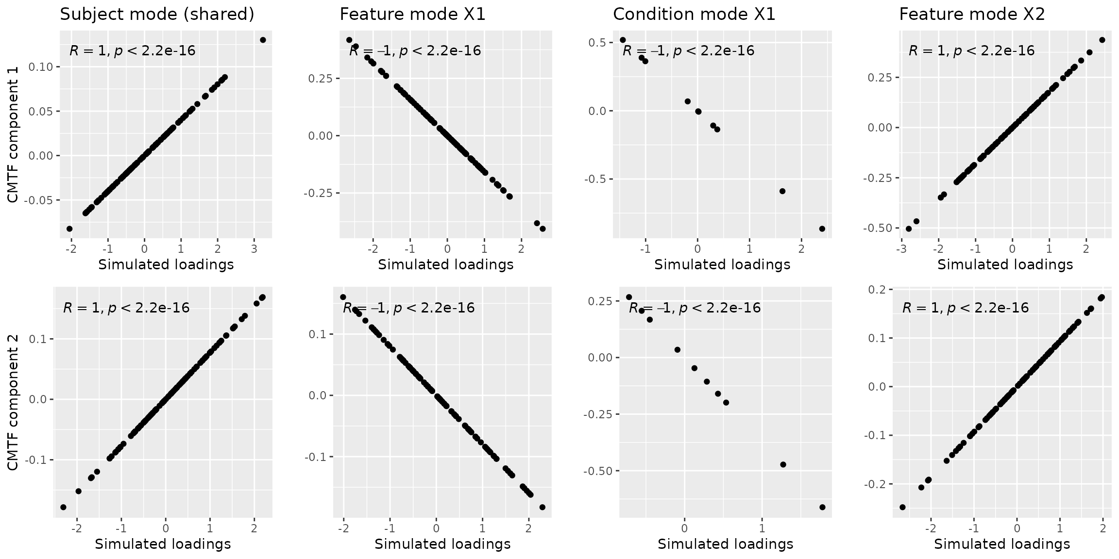 Note that negative correlations may be observed due to component
flipping, which is similar to Principal Component Analysis and does not
alter the description of the found subspace. There is also a difference
in magnitude between the simulated components and the modelled
components due to CMTF not penalizing the size of the vectors.
Note that negative correlations may be observed due to component
flipping, which is similar to Principal Component Analysis and does not
alter the description of the found subspace. There is also a difference
in magnitude between the simulated components and the modelled
components due to CMTF not penalizing the size of the vectors.
General two-tensor case
We create two tensor datasets sharing a subject mode with randomly initialized loadings corresponding to two components.
twoTensorData = simTwoTensorData(I=108, J=100, K=10, L=100, M=10, numComponents=2)We run the cmtf_opt() function using the two left vectors from an SVD of the tensors as our initial guess. This finds the correct solution pretty quickly.
result_nvec = cmtf_opt(twoTensorData$Z, 2, initialization="nvec")The f-value in result corresponds to the CMTF loss function value, which is very low in our case: 6.671611^{-9}. This solution was found using 22 iterations. We will visually verify this result with the plot below.
a = cbind(twoTensorData$A, result_nvec$Fac[[1]]) %>% as_tibble() %>% ggplot(aes(x=V2,y=V3)) + geom_point() + xlab("Simulated loadings") + ylab("CMTF component 1") + ggtitle("Subject mode (shared)") + stat_cor()
b = cbind(twoTensorData$B, result_nvec$Fac[[2]]) %>% as_tibble() %>% ggplot(aes(x=V2, y=V3)) + geom_point() + xlab("Simulated loadings") + ylab("") + ggtitle("Feature mode X1") + stat_cor()
c = cbind(twoTensorData$C, result_nvec$Fac[[3]]) %>% as_tibble() %>% ggplot(aes(x=V2,y=V3)) + geom_point() + xlab("Simulated loadings") + ylab("") + ggtitle("Condition mode X1") + stat_cor()
d = cbind(twoTensorData$D, result_nvec$Fac[[4]]) %>% as_tibble() %>% ggplot(aes(x=V2, y=V3)) + geom_point() + xlab("Simulated loadings") + ylab("") + ggtitle("Feature mode X2") + stat_cor()
e = cbind(twoTensorData$E, result_nvec$Fac[[5]]) %>% as_tibble() %>% ggplot(aes(x=V2,y=V3)) + geom_point() + xlab("Simulated loadings") + ylab("") + ggtitle("Condition mode X2") + stat_cor()
f = cbind(twoTensorData$A, result_nvec$Fac[[1]]) %>% as_tibble() %>% ggplot(aes(x=V1,y=V4)) + geom_point() + xlab("Simulated loadings") + ylab("CMTF component 2") + stat_cor()
g = cbind(twoTensorData$B, result_nvec$Fac[[2]]) %>% as_tibble() %>% ggplot(aes(x=V1, y=V4)) + geom_point() + xlab("Simulated loadings") + ylab("") + stat_cor()
h = cbind(twoTensorData$C, result_nvec$Fac[[3]]) %>% as_tibble() %>% ggplot(aes(x=V1,y=V4)) + geom_point() + xlab("Simulated loadings") + ylab("") + stat_cor()
i = cbind(twoTensorData$D, result_nvec$Fac[[4]]) %>% as_tibble() %>% ggplot(aes(x=V1, y=V4)) + geom_point() + xlab("Simulated loadings") + ylab("") + stat_cor()
j = cbind(twoTensorData$E, result_nvec$Fac[[5]]) %>% as_tibble() %>% ggplot(aes(x=V1,y=V4)) + geom_point() + xlab("Simulated loadings") + ylab("") + stat_cor()
ggarrange(a,b,c,d,e,f,g,h,i,j, nrow=2, ncol=5)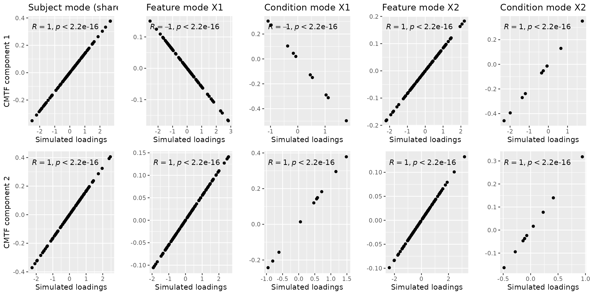 Note that negative correlations may be observed due to component
flipping, which is similar to Principal Component Analysis and does not
alter the description of the found subspace. There is also a difference
in magnitude between the simulated components and the modelled
components due to CMTF not penalizing the size of the vectors.
Note that negative correlations may be observed due to component
flipping, which is similar to Principal Component Analysis and does not
alter the description of the found subspace. There is also a difference
in magnitude between the simulated components and the modelled
components due to CMTF not penalizing the size of the vectors.
This concludes a brief introduction into applying cmtf_opt to various types of data. For a more in-depth analysis of robustness towards noise, we refer to Acar et al., 2011, which provides a framework that we replicate in the CMTF_noise_simulation vignette.