Introduction
This article presents the CP results of the AP dataset discussed in Chapter 7 of my dissertation.
Preamble
##
## Attaching package: 'dplyr'
## The following objects are masked from 'package:stats':
##
## filter, lag## The following objects are masked from 'package:base':
##
## intersect, setdiff, setequal, union##
## Attaching package: 'CMTFtoolbox'## The following object is masked from 'package:NPLStoolbox':
##
## npred## The following objects are masked from 'package:parafac4microbiome':
##
## fac_to_vect, reinflateFac, reinflateTensor, vect_to_fac
testMetadata = function(model, comp, metadata){

  transformedSubjectLoadings = model$Fac[[1]][,comp]
  transformedSubjectLoadings = transformedSubjectLoadings / norm(transformedSubjectLoadings, "2")

  metadata = metadata$mode1 %>% left_join(ageInfo, by="SubjectID") %>% mutate(Gender=as.numeric(as.factor(Gender), PainS_NopainA=as.numeric(as.factor(PainS_NopainA))))
  result = lm(transformedSubjectLoadings ~ Gender + Age + PainS_NopainA, data=metadata)

  # Extract coefficients and confidence intervals
  coef_estimates <- summary(result)$coefficients
  conf_intervals <- confint(result)

  # Remove intercept
  coef_estimates <- coef_estimates[rownames(coef_estimates) != "(Intercept)", ]
  conf_intervals <- conf_intervals[rownames(conf_intervals) != "(Intercept)", ]

  # Combine into a clean data frame
  summary_table <- data.frame(
    Term     = rownames(coef_estimates),
    Estimate = coef_estimates[, "Estimate"] * 1e3,
    CI       = paste0(
                 conf_intervals[, 1], " – ",
                 conf_intervals[, 2]
               ),
    P_value  = coef_estimates[, "Pr(>|t|)"],
    P_adjust = p.adjust(coef_estimates[, "Pr(>|t|)"], "BH"),
    row.names = NULL
  )

  return(summary_table)
}
cytokines_meta_data = read.csv("./AP/input_deduplicated_metadata_RvdP.csv", sep=" ", header=FALSE) %>% as_tibble()
colnames(cytokines_meta_data) = c("SubjectID", "Visit", "Gender", "Age", "Pain_noPain", "case_control")
ageInfo = cytokines_meta_data %>% select(SubjectID, Age) %>% unique()
# Case only subcohort
processedCytokines_case = CMTFtoolbox::Georgiou2025$Inflammatory_mediators

mask = processedCytokines_case$mode1$case_control == "case"
processedCytokines_case$data = processedCytokines_case$data[mask,,]
processedCytokines_case$mode1 = processedCytokines_case$mode1[mask,]

# Also remove subject A11-8 due to being an outlier
processedCytokines_case$data = processedCytokines_case$data[-25,,]
processedCytokines_case$mode1 = processedCytokines_case$mode1[-25,]

processedCytokines_case$data = log(processedCytokines_case$data + 0.005)
processedCytokines_case$data = multiwayCenter(processedCytokines_case$data, 1)
processedCytokines_case$data = multiwayScale(processedCytokines_case$data, 2)Inflammatory mediators
CP was applied to capture the dominant source of variation within the longitudinally measured inflammatory mediator data block. The model selection procedure indicates that CORCONDIA scores were inconclusive and loadings were unstable using four CP components. The commented code below performs the procedure, and is not rerun here due to computational limitations.
# assessment_cytokines_case = parafac4microbiome::assessModelQuality(processedCytokines_case$data, numRepetitions=10, numCores=10)
# assessment_cytokines_case$plots$overview
# assessment_cytokines_case$metrics$CORCONDIA %>% as_tibble() %>% mutate(index=1:nrow(.)) %>% pivot_longer(-index) %>% ggplot(aes(x=as.factor(name),y=value)) + geom_boxplot() + xlab("Number of components") + ylab("CORCONDIA") + theme(text=element_text(size=16))

# stability_cytokines = parafac4microbiome::assessModelStability(processedCytokines_case, maxNumComponents=5, numFolds=10, colourCols=colourCols, legendTitles=legendTitles, xLabels = xLabels, legendColNums=legendColNums, arrangeModes=arrangeModes, numCores=parallel::detectCores())
# stability_cytokines$modelPlots[[2]]
# stability_cytokines$modelPlots[[3]]
# stability_cytokines$modelPlots[[4]]
# stability_cytokines$modelPlots[[5]]
# cp_cytokines_case = parafac4microbiome::parafac(processedCytokines_case$data, nfac=3, nstart=100)
cp_cytokines_case = readRDS("./AP/cp_cytokines_case.RDS")

cp_cytokines_case$varExp
## [1] 36.56742Therefore, a three-component CP model was selected, explaining 36.6% of the variation. MLR analysis revealed that the first CP component captured variation associated with subject gender, while the second component was not interpretable, and the third component captured variation associated with a mixture of age and pain perception.
testMetadata(cp_cytokines_case, 1, processedCytokines_case)## Term Estimate CI
## 1 Gender 164.949044 0.0072276098315647 – 0.322670478266166
## 2 Age -1.993531 -0.00749714837460696 – 0.00351008731927873
## 3 PainS_NopainAS 90.764635 -0.0677608834293364 – 0.249290152970497
## P_value P_adjust
## 1 0.04120853 0.1236256
## 2 0.45964329 0.4596433
## 3 0.24705950 0.3705893
testMetadata(cp_cytokines_case, 2, processedCytokines_case)## Term Estimate CI P_value
## 1 Gender -10.645881 -0.188082738359188 – 0.166790975410106 0.9018900
## 2 Age -3.055744 -0.00924732264771653 – 0.0031358344938848 0.3164014
## 3 PainS_NopainAS 31.654457 -0.146686995485999 – 0.209995909725848 0.7157353
## P_adjust
## 1 0.90189
## 2 0.90189
## 3 0.90189
testMetadata(cp_cytokines_case, 3, processedCytokines_case)## Term Estimate CI
## 1 Gender 97.432563 -0.0307466851714757 – 0.225611811849372
## 2 Age -8.817799 -0.0132905554470071 – -0.00434504207134558
## 3 PainS_NopainAS -141.890668 -0.270723390978273 – -0.0130579456514781
## P_value P_adjust
## 1 0.1288756411 0.128875641
## 2 0.0005117721 0.001535316
## 3 0.0324479469 0.048671920
# Check sign
topIndices = processedCytokines_case$mode2 %>% mutate(index=1:nrow(.), Comp = cp_cytokines_case$Fac[[2]][,1]) %>% arrange(desc(Comp)) %>% head() %>% select(index) %>% pull()
bottomIndices = processedCytokines_case$mode2 %>% mutate(index=1:nrow(.), Comp = cp_cytokines_case$Fac[[2]][,1]) %>% arrange(desc(Comp)) %>% tail() %>% select(index) %>% pull()

Xhat = parafac4microbiome::reinflateTensor(cp_cytokines_case$Fac[[1]][,1], cp_cytokines_case$Fac[[2]][,1], cp_cytokines_case$Fac[[3]][,1])

print("Positive loadings:")
## [1] "Positive loadings:"
print(cor(Xhat[,topIndices[1],2], as.numeric(as.factor(processedCytokines_case$mode1$Gender)), use="pairwise.complete.obs")) # flip## [1] -0.4193432
print("Negative loadings:")## [1] "Negative loadings:"
print(cor(Xhat[,bottomIndices[5],2], as.numeric(as.factor(processedCytokines_case$mode1$Gender)), use="pairwise.complete.obs"))## [1] 0.4193432
# Plot
a = processedCytokines_case$mode1 %>%
  mutate(Comp1 = cp_cytokines_case$Fac[[1]][,1]) %>%
  ggplot(aes(x=as.factor(Gender),y=Comp1)) +
  geom_boxplot() +
  geom_jitter(height=0, width=0.05) +
  stat_compare_means(comparisons=list(c("F", "M")),label="p.signif") +
  xlab("") +
  ylab("Loading") +
  scale_x_discrete(labels=c("Female", "Male")) +
  theme(text=element_text(size=16))

temp = processedCytokines_case$mode2 %>%
  as_tibble() %>%
  mutate(Component_1 = -1*cp_cytokines_case$Fac[[2]][,1]) %>%
  arrange(Component_1) %>%
  mutate(index=1:nrow(.))

b=temp %>%
  ggplot(aes(x=as.factor(index),y=Component_1)) +
  geom_bar(stat="identity",col="black") +
  scale_x_discrete(label=temp$name) +
  xlab("") +
  ylab("Loading") +
  scale_x_discrete(labels=c("IL-10", "OPG", "VEGF", "CRP", expression(IFN-gamma), "IL-6", expression(TNF-alpha), "GM-CSF", "IL-17A", "IL-8", "IL-12p70", expression(IL-1*alpha), expression(IL-1*beta), expression(MIP-1*alpha), "IL-4", "RANKL")) +
  theme(text=element_text(size=16),axis.text.x = element_text(angle = 90, vjust = 0.5, hjust=1))
## Scale for x is already present.
## Adding another scale for x, which will replace the existing scale.
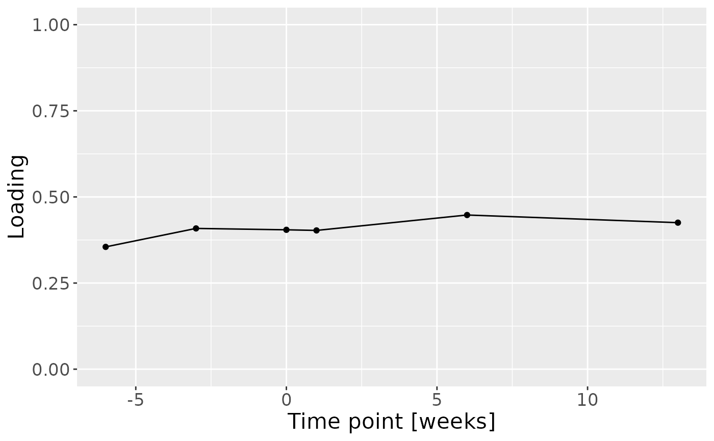
c = cp_cytokines_case$Fac[[3]][,1] %>% as_tibble() %>% mutate(value=-1*value) %>% mutate(timepoint=c(-6,-3,0,1,6,13)) %>% ggplot(aes(x=timepoint,y=value)) + geom_line() + geom_point() + xlab("Time point [weeks]") + ylab("Loading") + ylim(0,1) + theme(text=element_text(size=16))

a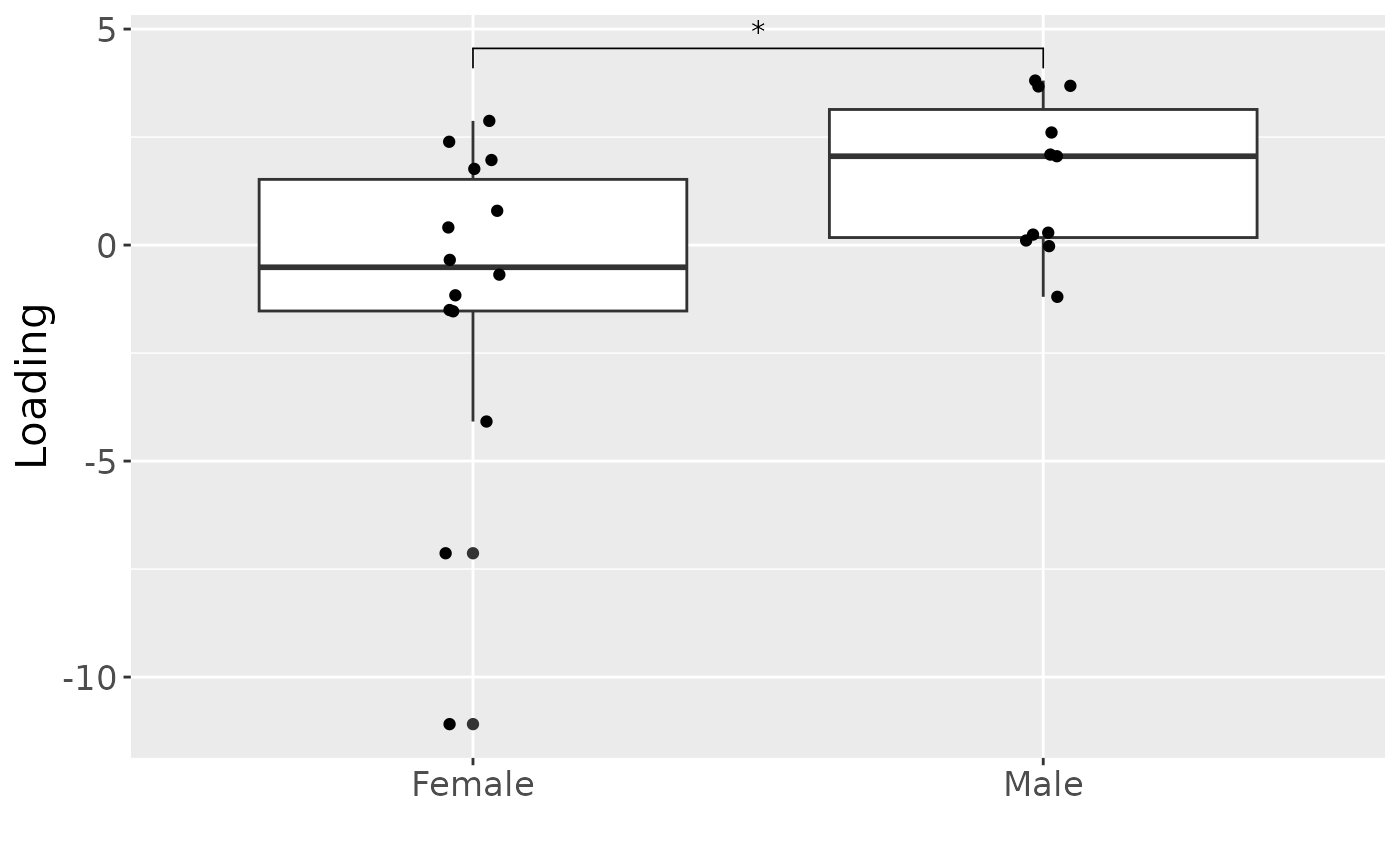
b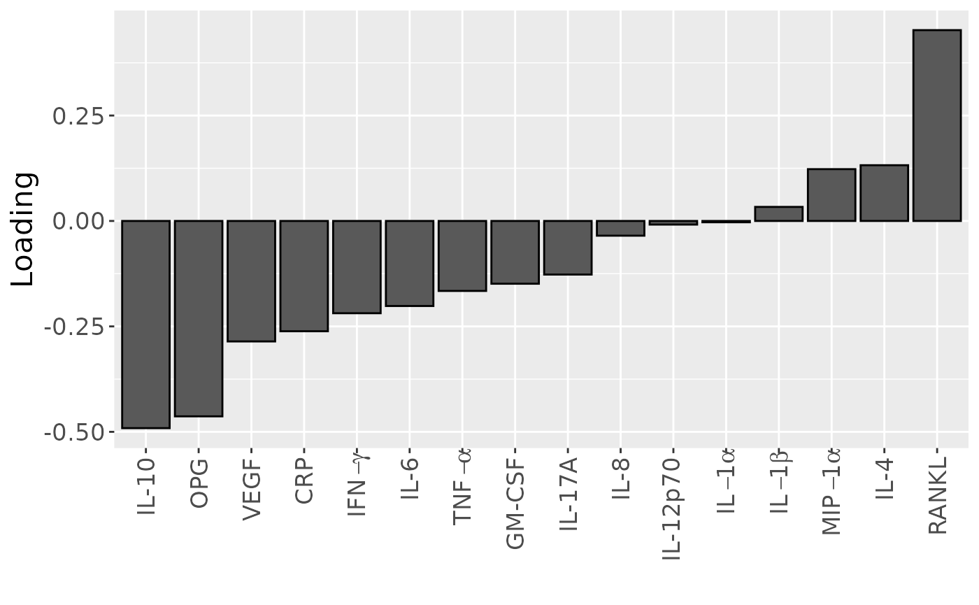
c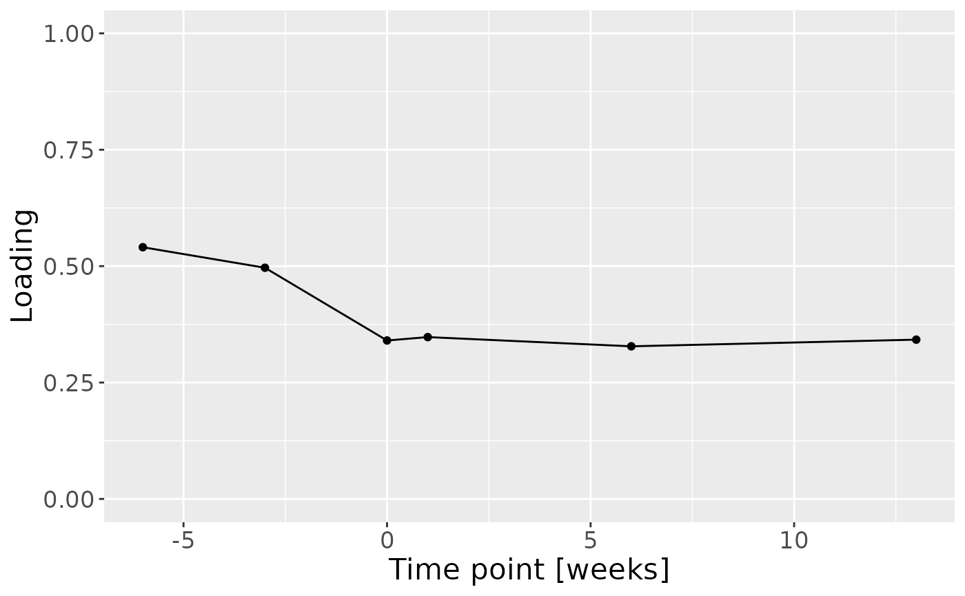
# Check sign
topIndices = processedCytokines_case$mode2 %>% mutate(index=1:nrow(.), Comp = cp_cytokines_case$Fac[[2]][,3]) %>% arrange(desc(Comp)) %>% head() %>% select(index) %>% pull()
bottomIndices = processedCytokines_case$mode2 %>% mutate(index=1:nrow(.), Comp = cp_cytokines_case$Fac[[2]][,3]) %>% arrange(desc(Comp)) %>% tail() %>% select(index) %>% pull()

Xhat = parafac4microbiome::reinflateTensor(cp_cytokines_case$Fac[[1]][,3], cp_cytokines_case$Fac[[2]][,3], cp_cytokines_case$Fac[[3]][,3])

print("Positive loadings:")
## [1] "Positive loadings:"
print(cor(Xhat[,topIndices[1],2], processedCytokines_case$mode1 %>% left_join(ageInfo) %>% select(Age), use="pairwise.complete.obs")) # no flip## Joining with `by = join_by(SubjectID)`## Age
## [1,] 0.5797891
print("Negative loadings:")## [1] "Negative loadings:"
print(cor(Xhat[,bottomIndices[5],2], processedCytokines_case$mode1 %>% left_join(ageInfo) %>% select(Age), use="pairwise.complete.obs"))## Joining with `by = join_by(SubjectID)`## Age
## [1,] -0.5797891
# Plot
a = processedCytokines_case$mode1 %>%
  left_join(ageInfo) %>%
  mutate(Comp1 = cp_cytokines_case$Fac[[1]][,3]) %>%
  ggplot(aes(x=Age,y=Comp1)) +
  geom_point() +
  stat_cor() +
  xlab("Age") +
  ylab("Loading") +
  theme(text=element_text(size=16))
## Joining with `by = join_by(SubjectID)`
temp = processedCytokines_case$mode2 %>%
  as_tibble() %>%
  mutate(Component_1 = cp_cytokines_case$Fac[[2]][,3]) %>%
  arrange(Component_1) %>%
  mutate(index=1:nrow(.))

b=temp %>%
  ggplot(aes(x=as.factor(index),y=Component_1)) +
  geom_bar(stat="identity",col="black") +
  scale_x_discrete(label=temp$name) +
  xlab("") +
  ylab("Loading") +
  scale_x_discrete(labels=c("IL-10", "IL-17A", "GM-CSF", "IL-12p70", expression(IFN-gamma), expression(IL-1*alpha), "RANKL", expression(IL-1*beta), "CRP", "OPG", expression(MIP-1*alpha), "IL-6", expression(TNF-alpha), "VEGF", "IL-8")) +
  theme(text=element_text(size=16),axis.text.x = element_text(angle = 90, vjust = 0.5, hjust=1))
## Scale for x is already present.
## Adding another scale for x, which will replace the existing scale.
c = cp_cytokines_case$Fac[[3]][,3] %>% as_tibble() %>% mutate(value=-1*value) %>% mutate(timepoint=c(-6,-3,0,1,6,13)) %>% ggplot(aes(x=timepoint,y=value)) + geom_line() + geom_point() + xlab("Time point [weeks]") + ylab("Loading") + ylim(0,1) + theme(text=element_text(size=16))

a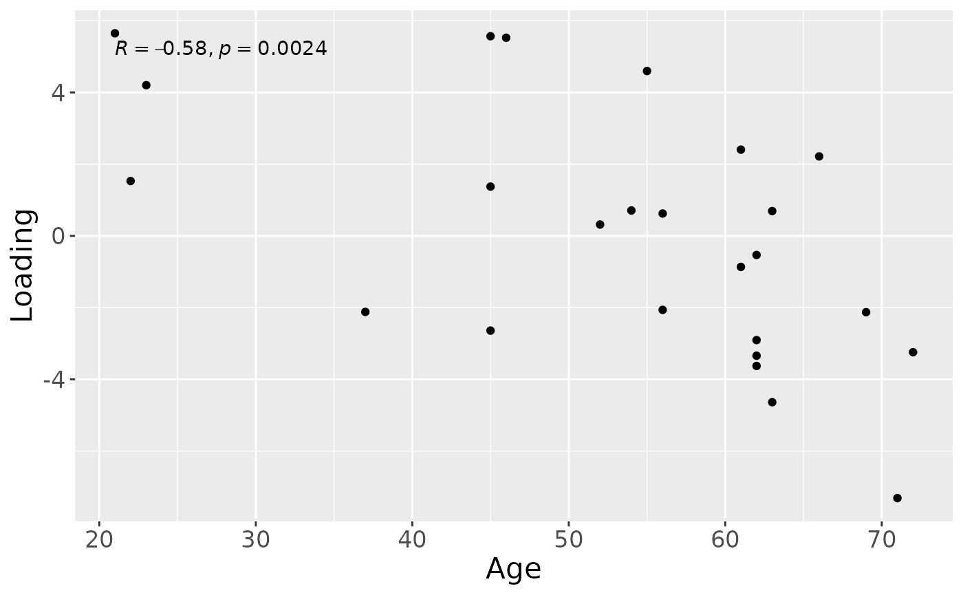
b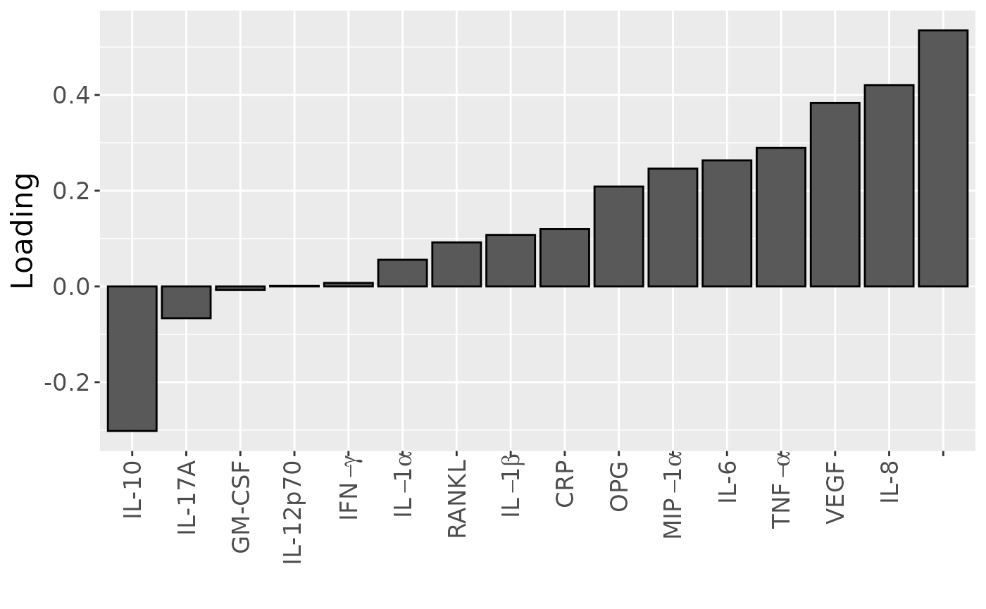
c