TIFN2: Red fluorescent plaque development in gingivitis
2025-08-31
Source:vignettes/articles/TIFN2.Rmd
TIFN2.RmdIntroduction
This article presents the CP results of the TIFN2 dataset discussed in Chapter 4 of my dissertation.
Preamble
##
## Attaching package: 'dplyr'
## The following objects are masked from 'package:stats':
##
## filter, lag## The following objects are masked from 'package:base':
##
## intersect, setdiff, setequal, union##
## Attaching package: 'CMTFtoolbox'## The following object is masked from 'package:NPLStoolbox':
##
## npred## The following objects are masked from 'package:parafac4microbiome':
##
## fac_to_vect, reinflateFac, reinflateTensor, vect_to_fac
rf_data = read.csv("../../data-raw/vanderPloeg2024/RFdata.csv")
colnames(rf_data) = c("subject", "id", "fotonr", "day", "group", "RFgroup", "MQH", "SPS(tm)", "Area_delta_R30", "Area_delta_Rmax", "Area_delta_R30_x_Rmax", "gingiva_mean_R_over_G", "gingiva_mean_R_over_G_upper_jaw", "gingiva_mean_R_over_G_lower_jaw")
rf_data = rf_data %>% as_tibble()

rf_data[rf_data$subject == "VSTPHZ", 1] = "VSTPH2"
rf_data[rf_data$subject == "D2VZH0", 1] = "DZVZH0"
rf_data[rf_data$subject == "DLODNN", 1] = "DLODDN"
rf_data[rf_data$subject == "O3VQFX", 1] = "O3VQFQ"
rf_data[rf_data$subject == "F80LGT", 1] = "F80LGF"
rf_data[rf_data$subject == "26QQR0", 1] = "26QQrO"

rf_data2 = read.csv("../../data-raw/vanderPloeg2024/red_fluorescence_data.csv") %>% as_tibble()
rf_data2 = rf_data2[,c(2,4,181:192)]
rf_data = rf_data %>% left_join(rf_data2)
## Joining with `by = join_by(id, day)`
age_gender = read.csv("../../data-raw/vanderPloeg2024/Ploeg_subjectMetadata.csv", sep=";")
age_gender = age_gender[2:nrow(age_gender),2:ncol(age_gender)]
age_gender = age_gender %>% as_tibble() %>% filter(onderzoeksgroep == 0) %>% select(naam, leeftijd, geslacht)
colnames(age_gender) = c("subject", "age", "gender")

# Correction for incorrect subject ids
age_gender[age_gender$subject == "VSTPHZ", 1] = "VSTPH2"
age_gender[age_gender$subject == "D2VZH0", 1] = "DZVZH0"
age_gender[age_gender$subject == "DLODNN", 1] = "DLODDN"
age_gender[age_gender$subject == "O3VQFX", 1] = "O3VQFQ"
age_gender[age_gender$subject == "F80LGT", 1] = "F80LGF"
age_gender[age_gender$subject == "26QQR0", 1] = "26QQrO"

age_gender = age_gender %>% arrange(subject)
mapping = c(-14,0,2,5,9,14,21)

testMetadata = function(model, comp, metadata){
  transformedSubjectLoadings = model$Fac[[1]][,comp]
  transformedSubjectLoadings = transformedSubjectLoadings / norm(transformedSubjectLoadings, "2")

  metadata = metadata$mode1 %>% left_join(rf_data %>% select(subject,day,Area_delta_R30,plaquepercent,bomppercent) %>% filter(day==14), by="subject")

  result = lm(transformedSubjectLoadings ~ plaquepercent + bomppercent + Area_delta_R30 + gender + age, data=metadata)

  # Extract coefficients and confidence intervals
  coef_estimates <- summary(result)$coefficients
  conf_intervals <- confint(result)

  # Remove intercept
  coef_estimates <- coef_estimates[rownames(coef_estimates) != "(Intercept)", ]
  conf_intervals <- conf_intervals[rownames(conf_intervals) != "(Intercept)", ]

  # Combine into a clean data frame
  summary_table <- data.frame(
    Term     = rownames(coef_estimates),
    Estimate = coef_estimates[, "Estimate"] * 1e3,
    CI       = paste0(
                 conf_intervals[, 1], " – ",
                 conf_intervals[, 2]
               ),
    P_value  = coef_estimates[, "Pr(>|t|)"],
    P_adjust = p.adjust(coef_estimates[, "Pr(>|t|)"], "BH"),
    row.names = NULL
  )

  return(summary_table)
}

testFeatures = function(model, metadata, componentNum, metadataVar){
  df = metadata$mode1 %>% left_join(rf_data %>% filter(day==14)) %>% left_join(age_gender)
  topIndices = metadata$mode2 %>% mutate(index=1:nrow(.), Comp = model$Fac[[2]][,componentNum]) %>% arrange(desc(Comp)) %>% head() %>% select(index) %>% pull()
  bottomIndices = metadata$mode2 %>% mutate(index=1:nrow(.), Comp = model$Fac[[2]][,componentNum]) %>% arrange(desc(Comp)) %>% tail() %>% select(index) %>% pull()

  timepoint = which(abs(model$Fac[[3]][,componentNum]) == max(abs(model$Fac[[3]][,componentNum])))

  Xhat = parafac4microbiome::reinflateTensor(model$Fac[[1]][,componentNum], model$Fac[[2]][,componentNum], model$Fac[[3]][,componentNum])
  y = df[metadataVar]

  print("Positive loadings:")
  print(cor(Xhat[,topIndices[1],timepoint], y))
  print("Negative loadings:")
  print(cor(Xhat[,bottomIndices[1],timepoint], y))
}

plotFeatures = function(mode2, model, componentNum, flip=FALSE){

  if(flip==TRUE){
    df = mode2 %>% mutate(Comp = -1*model$Fac[[2]][,componentNum]) %>% arrange(Comp) %>% filter(Species != "") %>% mutate(index=1:nrow(.), name = paste(Genus, Species))
  } else{
    df = mode2 %>% mutate(Comp = model$Fac[[2]][,componentNum]) %>% arrange(Comp) %>% filter(Species != "") %>% mutate(index=1:nrow(.), name = paste(Genus, Species))
  }
  df = rbind(df %>% head(n=10), df %>% tail(n=10))

  plot=df %>%
    ggplot(aes(x=Comp,y=as.factor(index),fill=as.factor(Phylum))) +
    geom_bar(stat="identity", col="black") +
    scale_y_discrete(label=df$name) +
    xlab("Loading") +
    ylab("") +
    guides(fill=guide_legend(title="Phylum")) +
    theme(text=element_text(size=16))

  return(plot)
}
phylum_colors = hue_pal()(7)
processedTongue = processDataCube(parafac4microbiome::vanderPloeg2024$tongue, sparsityThreshold=0.50, considerGroups=TRUE, groupVariable="RFgroup", CLR=TRUE, centerMode=1, scaleMode=2)
processedLowling = processDataCube(parafac4microbiome::vanderPloeg2024$lower_jaw_lingual, sparsityThreshold=0.50, considerGroups=TRUE, groupVariable="RFgroup", CLR=TRUE, centerMode=1, scaleMode=2)
processedLowinter = processDataCube(parafac4microbiome::vanderPloeg2024$lower_jaw_interproximal, sparsityThreshold=0.50, considerGroups=TRUE, groupVariable="RFgroup", CLR=TRUE, centerMode=1, scaleMode=2)
processedUpling = processDataCube(parafac4microbiome::vanderPloeg2024$upper_jaw_lingual, sparsityThreshold=0.50, considerGroups=TRUE, groupVariable="RFgroup", CLR=TRUE, centerMode=1, scaleMode=2)
processedUpinter = processDataCube(parafac4microbiome::vanderPloeg2024$upper_jaw_interproximal, sparsityThreshold=0.50, considerGroups=TRUE, groupVariable="RFgroup", CLR=TRUE, centerMode=1, scaleMode=2)
processedSaliva = processDataCube(parafac4microbiome::vanderPloeg2024$saliva, sparsityThreshold=0.50, considerGroups=TRUE, groupVariable="RFgroup", CLR=TRUE, centerMode=1, scaleMode=2)
processedMetabolomics = parafac4microbiome::vanderPloeg2024$metabolomicsTongue microbiome
CP was applied to capture the dominant source of variation in the tongue microbiome data block. The model selection procedure revealed that CORCONDIA scores were inconclusive and loadings were unstable at three components. The commented code below performs the procedure, and is not rerun here due to computational limitations.
# assessment_tongue = parafac4microbiome::assessModelQuality(processedTongue$data, numRepetitions=10, numCores=10)

# assessment_tongue$metrics$CORCONDIA %>% as_tibble() %>% mutate(index=1:nrow(.)) %>% pivot_longer(-index) %>% ggplot(aes(x=as.factor(name),y=value)) + geom_boxplot() + xlab("Number of components") + ylab("CORCONDIA") + theme(text=element_text(size=16))

# stability_tongue = parafac4microbiome::assessModelStability(processedTongue, maxNumComponents=3, numFolds=10, colourCols=colourCols, legendTitles=legendTitles, xLabels = xLabels, legendColNums=legendColNums, arrangeModes=arrangeModes, numCores=parallel::detectCores())
# stability_tongue$modelPlots[[2]]
# stability_tongue$modelPlots[[3]]
# cp_tongue = parafac4microbiome::parafac(processedTongue$data, nfac=2, nstart=100)

cp_tongue = readRDS("./TIFN2/cp_tongue.RDS")
cp_tongue$varExp
## [1] 31.37847Therefore, a two-component CP model was selected, explaining 31.4% of the variation. However, MLR analysis revealed that the first component captured variation associated with a mixture of plaque% and subject age, while the second component was not interpretable.
testMetadata(cp_tongue, 1, processedTongue)## Term Estimate CI
## 1 plaquepercent -7.085726 -0.0125436561188763 – -0.00162779504204587
## 2 bomppercent 1.189991 -0.00221993077742614 – 0.00459991246706438
## 3 Area_delta_R30 2.527468 -0.00434891510321956 – 0.00940385109507837
## 4 gender 11.109220 -0.0857143066863078 – 0.107932746588392
## 5 age 13.793423 0.00516939627811755 – 0.0224174495211815
## P_value P_adjust
## 1 0.012433782 0.03108445
## 2 0.483348754 0.60418594
## 3 0.460540316 0.60418594
## 4 0.817174114 0.81717411
## 5 0.002572981 0.01286491
testMetadata(cp_tongue, 2, processedTongue)## Term Estimate CI
## 1 plaquepercent -0.877180 -0.00719453415388883 – 0.00544017410099945
## 2 bomppercent -2.057600 -0.0060044593190253 – 0.00188925874240208
## 3 Area_delta_R30 -5.035993 -0.012995154144287 – 0.00292316758866404
## 4 gender -42.102114 -0.154171789877283 – 0.0699675615970461
## 5 age 2.246435 -0.00773555910142959 – 0.0122284290033156
## P_value P_adjust
## 1 0.7796915 0.7796915
## 2 0.2971467 0.7428669
## 3 0.2074012 0.7428669
## 4 0.4507719 0.7512864
## 5 0.6505852 0.7796915
testFeatures(cp_tongue, processedTongue, 1, "plaquepercent") # no flip## Joining with `by = join_by(subject, RFgroup)`
## Joining with `by = join_by(subject, age, gender)`## [1] "Positive loadings:"
## plaquepercent
## [1,] 0.3063565
## [1] "Negative loadings:"
## plaquepercent
## [1,] -0.3063565
testFeatures(cp_tongue, processedTongue, 1, "age") # flip## Joining with `by = join_by(subject, RFgroup)`
## Joining with `by = join_by(subject, age, gender)`## [1] "Positive loadings:"
## age
## [1,] -0.4538388
## [1] "Negative loadings:"
## age
## [1,] 0.4538388
a = processedTongue$mode1 %>%
  mutate(Component_1 = cp_tongue$Fac[[1]][,1]) %>%
  left_join(rf_data %>% select(subject,day,Area_delta_R30,plaquepercent,bomppercent) %>% filter(day==14), by="subject") %>%
  ggplot(aes(x=plaquepercent,y=Component_1)) +
  geom_point() +
  xlab("Plaque%") +
  ylab("Loading") +
  stat_cor() +
  theme(text=element_text(size=16))

b = plotFeatures(processedTongue$mode2, cp_tongue, 1, flip=FALSE) + scale_fill_manual(values=phylum_colors[-c(3,7)]) + theme(legend.position="none")

c = processedTongue$mode3 %>%
  mutate(Component_1 = -1*cp_tongue$Fac[[3]][,1], day=c(-14,0,2,5,9,14,21)) %>%
  ggplot(aes(x=day,y=Component_1)) +
  annotate(geom = "rect", xmin = 0, xmax = 14, ymin = -Inf, ymax = Inf, fill = "red", colour = "black", alpha=0.25) +
  geom_line() +
  geom_point() +
  xlab("Time point [days]") +
  ylab("Loading") +
  ylim(0,1) +
  theme(legend.position="none", text=element_text(size=16))

a
b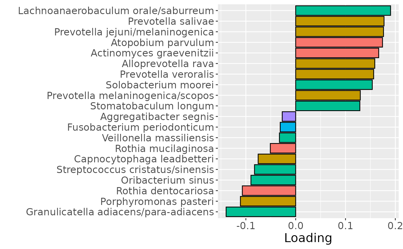
c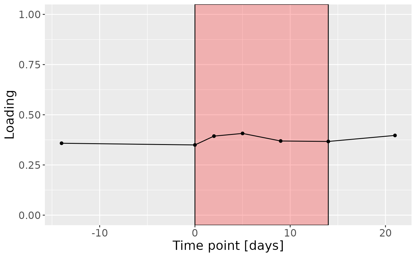
Lower jaw lingual microbiome
CP was applied to capture the dominant source of variation in the lower jaw lingual microbiome data block. The model selection procedure revealed CORCONDIA scores were too low at two components. The commented code below performs the procedure, and is not rerun here due to computational limitations.
# assessment_lowling = parafac4microbiome::assessModelQuality(processedLowling$data, numRepetitions=10, numCores=10)

# assessment_lowling$metrics$CORCONDIA %>% as_tibble() %>% mutate(index=1:nrow(.)) %>% pivot_longer(-index) %>% ggplot(aes(x=as.factor(name),y=value)) + geom_boxplot() + xlab("Number of components") + ylab("CORCONDIA") + theme(text=element_text(size=16))

# stability_lowling = parafac4microbiome::assessModelStability(processedLowling, maxNumComponents=2, numFolds=10, colourCols=colourCols, legendTitles=legendTitles, xLabels = xLabels, legendColNums=legendColNums, arrangeModes=arrangeModes, numCores=parallel::detectCores())
# stability_lowling$modelPlots[[1]]
# stability_lowling$modelPlots[[2]]
# cp_lowling = parafac4microbiome::parafac(processedLowling$data, nfac=1, nstart=100)
cp_lowling = readRDS("./TIFN2/cp_lowling.RDS")

cp_lowling$varExp
## [1] 10.55114Therefore, a one-component CP model was selected, explaining 10.6% of the variation. Surprisingly, MLR analysis revealed that the CP component captured variation exclusively associated with RF%.
testMetadata(cp_lowling, 1, processedLowling)## Term Estimate CI
## 1 plaquepercent -4.047703 -0.00897953402999654 – 0.000884127338494313
## 2 bomppercent -2.597078 -0.00567831104112229 – 0.000484155105742315
## 3 Area_delta_R30 -10.235675 -0.0164492308704168 – -0.00402211882627686
## 4 gender -83.222465 -0.170712996229106 – 0.00426806527981913
## 5 age -2.544554 -0.0103372952848458 – 0.0052481867268659
## P_value P_adjust
## 1 0.10460587 0.130757338
## 2 0.09591003 0.130757338
## 3 0.00197737 0.009886849
## 4 0.06160528 0.130757338
## 5 0.51174413 0.511744134
testFeatures(cp_lowling, processedLowling, 1, "Area_delta_R30") # flip## Joining with `by = join_by(subject, RFgroup)`
## Joining with `by = join_by(subject, age, gender)`## [1] "Positive loadings:"
## Area_delta_R30
## [1,] -0.5298343
## [1] "Negative loadings:"
## Area_delta_R30
## [1,] 0.5298343
a = processedLowling$mode1 %>%
  mutate(Component_1 = cp_lowling$Fac[[1]][,1]) %>%
  left_join(rf_data %>% select(subject,day,Area_delta_R30,plaquepercent,bomppercent) %>% filter(day==14), by="subject") %>%
  ggplot(aes(x=Area_delta_R30,y=Component_1)) +
  geom_point() +
  xlab("RF%") +
  ylab("Loading") +
  stat_cor() +
  theme(text=element_text(size=16))

b = plotFeatures(processedLowling$mode2, cp_lowling, 1, flip=TRUE) + scale_fill_manual(values=phylum_colors[-7]) + theme(legend.position="none")

c = processedLowling$mode3 %>%
  mutate(Component_1 = cp_lowling$Fac[[3]][,1], day=c(-14,0,2,5,9,14,21)) %>%
  ggplot(aes(x=day,y=Component_1)) +
  annotate(geom = "rect", xmin = 0, xmax = 14, ymin = -Inf, ymax = Inf, fill = "red", colour = "black", alpha=0.25) +
  geom_line() +
  geom_point() +
  xlab("Time point [days]") +
  ylab("Loading") +
  ylim(0,1) +
  theme(legend.position="none", text=element_text(size=16))

a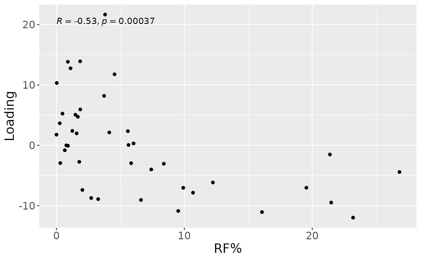
b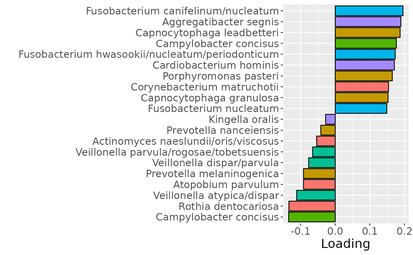
c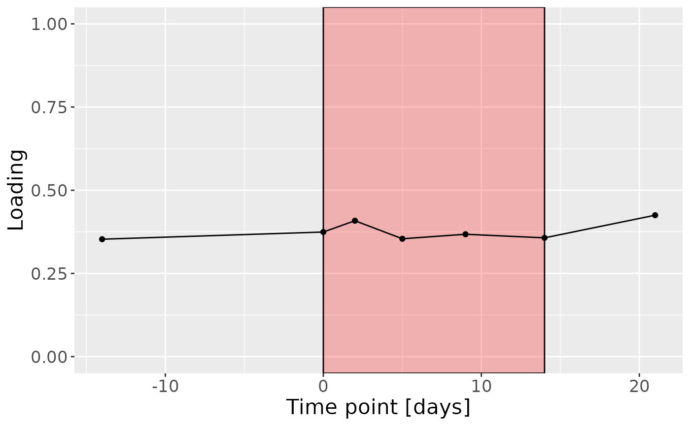
Positively loaded microbiota including Fusobacterium canifelinum / nucleatum, Aggregatibacter segnis, Capnocytophaga leadbetteri, Campylobacter concisus, Fusobacterium hwasookii / nucleatum / periodonticum, Cardiobacterium hominis, Porphyromonas pasteri, Corynebacterium matruchotii, Capnocytophaga granulosa, and Fusobacterium nucleatum were enriched in high responders and depleted in low responders. Conversely, negatively loaded microbiota including Campylobacter concisus, Rothia dentocariosa, Veillonella atypica / dispar, Atopobium parvulum, Prevotella melaninogenica, Veillonella dispar / parvula, Veillonella parvula / rogosae / tobetsuensis, Actinomyces naeslundii / oris / viscosus, Prevotella nanceiensis, and Kingella oralis were enriched in low responders and depleted in high responders. The time mode loadings of the component indicate that the inter-subject differences due to RF% were constant throughout the time series.
Lower jaw interproximal microbiome
CP was applied to capture the dominant source of variation in the lower jaw interproximal microbiome data block. The model selection procedure revealed that CORCONDIA scores were too low at three components. The commented code below performs the procedure, and is not rerun here due to computational limitations.
# assessment_lowinter = parafac4microbiome::assessModelQuality(processedLowinter$data, numRepetitions=10, numCores=10)

# assessment_lowinter$metrics$CORCONDIA %>% as_tibble() %>% mutate(index=1:nrow(.)) %>% pivot_longer(-index) %>% ggplot(aes(x=as.factor(name),y=value)) + geom_boxplot() + xlab("Number of components") + ylab("CORCONDIA") + theme(text=element_text(size=16))

#
# stability_lowinter = parafac4microbiome::assessModelStability(processedLowinter, maxNumComponents=3, numFolds=10, colourCols=colourCols, legendTitles=legendTitles, xLabels = xLabels, legendColNums=legendColNums, arrangeModes=arrangeModes, numCores=parallel::detectCores())
# stability_lowinter$modelPlots[[2]]
# stability_lowinter$modelPlots[[3]]
#
# cp_lowinter = parafac4microbiome::parafac(processedLowinter$data, nfac=2, nstart=100)
cp_lowinter = readRDS("./TIFN2/cp_lowinter.RDS")

cp_lowinter$varExp
## [1] 10.32969Therefore, a two-component CP model was selected, explaining 10.3% of the variation. However, MLR analysis revealed that the first CP component captured uninterpretable variation, while the second component captured variation exclusively associated with BOMP%.
testMetadata(cp_lowinter, 1, processedLowinter)## Term Estimate CI
## 1 plaquepercent -2.8231325 -0.00885260016583814 – 0.00320633515325942
## 2 bomppercent -3.6808351 -0.00744783286106304 – 8.61626701053834e-05
## 3 Area_delta_R30 -0.6104507 -0.00820690677640243 – 0.00698600534263869
## 4 gender -24.7799778 -0.131742556135758 – 0.0821826004540417
## 5 age -3.2188894 -0.0127459966584142 – 0.00630821784418125
## P_value P_adjust
## 1 0.34835493 0.8013102
## 2 0.05517984 0.2758992
## 3 0.87134707 0.8713471
## 4 0.64104814 0.8013102
## 5 0.49729155 0.8013102
testMetadata(cp_lowinter, 2, processedLowinter)## Term Estimate CI
## 1 plaquepercent 2.156444 -0.00382845328747255 – 0.0081413416846705
## 2 bomppercent -4.091747 -0.00783089859963512 – -0.000352594798941325
## 3 Area_delta_R30 7.257480 -0.000282823087328943 – 0.0147977821470906
## 4 gender 74.027343 -0.032144561763505 – 0.18019924770268
## 5 age 5.422361 -0.0040343211065686 – 0.0148790435409806
## P_value P_adjust
## 1 0.46935734 0.4693573
## 2 0.03287750 0.1468343
## 3 0.05873372 0.1468343
## 4 0.16576694 0.2762782
## 5 0.25228070 0.3153509
testFeatures(cp_lowinter, processedLowinter, 2, "bomppercent") # no flip## Joining with `by = join_by(subject, RFgroup)`
## Joining with `by = join_by(subject, age, gender)`## [1] "Positive loadings:"
## bomppercent
## [1,] 0.2341633
## [1] "Negative loadings:"
## bomppercent
## [1,] -0.2341633
a = processedLowinter$mode1 %>%
  mutate(Component_1 = cp_lowinter$Fac[[1]][,2]) %>%
  left_join(rf_data %>% select(subject,day,Area_delta_R30,plaquepercent,bomppercent) %>% filter(day==14), by="subject") %>%
  ggplot(aes(x=bomppercent,y=Component_1)) +
  geom_point() +
  xlab("BOMP%") +
  ylab("Loading") +
  stat_cor() +
  theme(text=element_text(size=16))

b = plotFeatures(processedLowinter$mode2, cp_lowinter, 2, flip=FALSE) + scale_fill_manual(values=phylum_colors[-c(3)]) + theme(legend.position="none")

c = processedLowinter$mode3 %>%
  mutate(Component_1 = -1*cp_lowinter$Fac[[3]][,2], day=c(-14,0,2,5,9,14,21)) %>%
  ggplot(aes(x=day,y=Component_1)) +
  annotate(geom = "rect", xmin = 0, xmax = 14, ymin = -Inf, ymax = Inf, fill = "red", colour = "black", alpha=0.25) +
  geom_line() +
  geom_point() +
  xlab("Time point [days]") +
  ylab("Loading") +
  ylim(0,1) +
  theme(legend.position="none", text=element_text(size=16))

a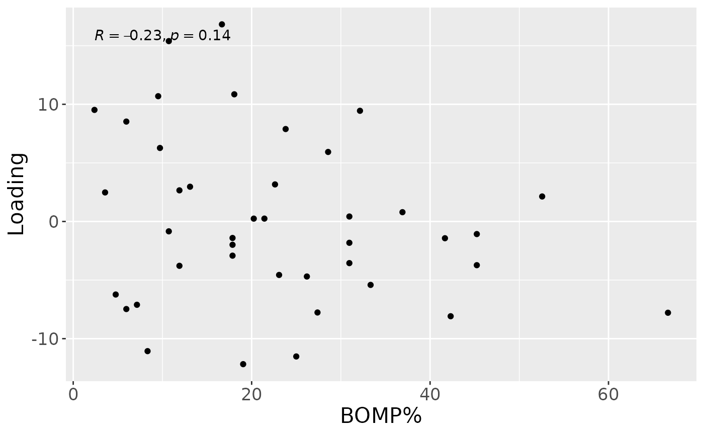
b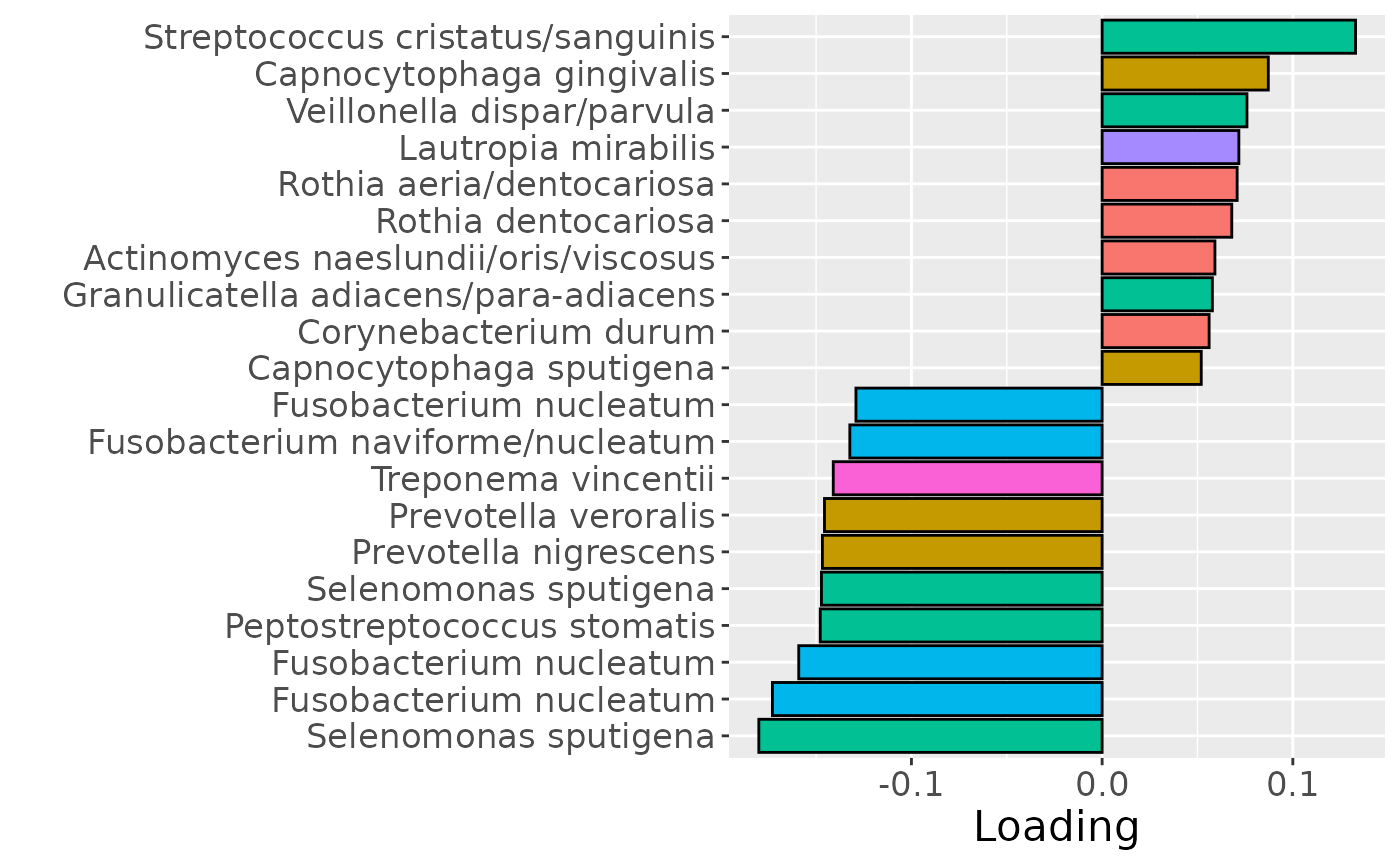
c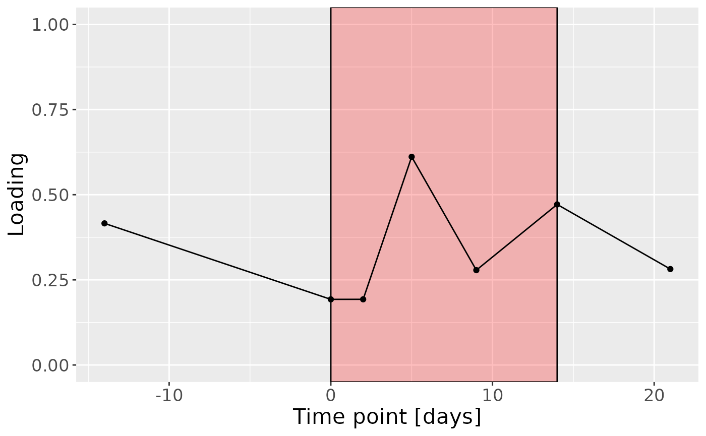
Upper jaw lingual microbiome
CP was applied to capture the dominant source of variation in the upper jaw lingual microbiome data block. The model selection procedure revealed that CORCONDIA scores were too low at three components. The commented code below performs the procedure, and is not rerun here due to computational limitations.
# assessment_upling = parafac4microbiome::assessModelQuality(processedUpling$data, numRepetitions=10, numCores=10)

# assessment_upling$metrics$CORCONDIA %>% as_tibble() %>% mutate(index=1:nrow(.)) %>% pivot_longer(-index) %>% ggplot(aes(x=as.factor(name),y=value)) + geom_boxplot() + xlab("Number of components") + ylab("CORCONDIA") + theme(text=element_text(size=16))

# stability_upling = parafac4microbiome::assessModelStability(processedUpling, maxNumComponents=3, numFolds=10, colourCols=colourCols, legendTitles=legendTitles, xLabels = xLabels, legendColNums=legendColNums, arrangeModes=arrangeModes, numCores=parallel::detectCores())
# stability_upling$modelPlots[[2]]
# stability_upling$modelPlots[[3]]
#
# cp_upling = parafac4microbiome::parafac(processedUpling$data, nfac=2, nstart=100)
cp_upling = readRDS("./TIFN2/cp_upling.RDS")

cp_upling$varExp
## [1] 19.19163Therefore, a two-component CP model was selected, explaining 19.2% of the variation. However, MLR analysis revealed that the first CP component captured uninterpretable variation, while the second component captured variation exclusively but weakly associated with RF%.
testMetadata(cp_upling, 1, processedUpling)## Term Estimate CI
## 1 plaquepercent 3.5957413 -0.00193167844376722 – 0.00912316112826477
## 2 bomppercent 2.5813448 -0.000871991211114323 – 0.00603468087307641
## 3 Area_delta_R30 7.9435166 0.000979584806484587 – 0.0149074483917542
## 4 gender 78.4426156 -0.0196136482063289 – 0.176498879470703
## 5 age -0.4196712 -0.00915349714410007 – 0.00831415476076494
## P_value P_adjust
## 1 0.19519152 0.2439894
## 2 0.13812418 0.2302070
## 3 0.02655809 0.1327905
## 4 0.11334141 0.2302070
## 5 0.92284676 0.9228468
testMetadata(cp_upling, 2, processedUpling)## Term Estimate CI
## 1 plaquepercent -2.5436852 -0.0086495593078846 – 0.00356218888854485
## 2 bomppercent -0.1702389 -0.0039849726780106 – 0.00364449492465157
## 3 Area_delta_R30 -8.1288343 -0.0158215539877252 – -0.000436114704840301
## 4 gender -85.1621897 -0.193480215958621 – 0.0231558365641216
## 5 age -0.6466179 -0.0102944542293067 – 0.00900121851702191
## P_value P_adjust
## 1 0.40344530 0.6724088
## 2 0.92832935 0.9283294
## 3 0.03895533 0.1947767
## 4 0.11945334 0.2986333
## 5 0.89255185 0.9283294
testFeatures(cp_upling, processedUpling, 2, "Area_delta_R30") # flip## Joining with `by = join_by(subject, RFgroup)`
## Joining with `by = join_by(subject, age, gender)`## [1] "Positive loadings:"
## Area_delta_R30
## [1,] -0.3280193
## [1] "Negative loadings:"
## Area_delta_R30
## [1,] 0.3280193
a = processedUpling$mode1 %>%
  mutate(Component_1 = cp_upling$Fac[[1]][,2]) %>%
  left_join(rf_data %>% select(subject,day,Area_delta_R30,plaquepercent,bomppercent) %>% filter(day==14), by="subject") %>%
  ggplot(aes(x=Area_delta_R30,y=Component_1)) +
  geom_point() +
  xlab("RF%") +
  ylab("Loading") +
  stat_cor() +
  theme(text=element_text(size=16))

b = plotFeatures(processedUpling$mode2, cp_upling, 2, flip=TRUE) + scale_fill_manual(values=phylum_colors[-c(3,7)]) + theme(legend.position="none")

c = processedUpling$mode3 %>%
  mutate(Component_1 = cp_upling$Fac[[3]][,2], day=c(-14,0,2,5,9,14,21)) %>%
  ggplot(aes(x=day,y=Component_1)) +
  annotate(geom = "rect", xmin = 0, xmax = 14, ymin = -Inf, ymax = Inf, fill = "red", colour = "black", alpha=0.25) +
  geom_line() +
  geom_point() +
  xlab("Time point [days]") +
  ylab("Loading") +
  ylim(0,1) +
  theme(legend.position="none", text=element_text(size=16))

a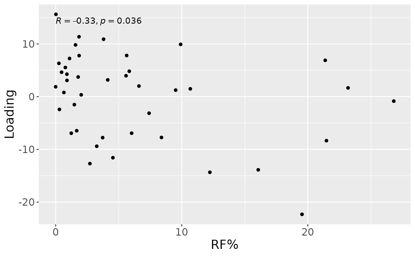
b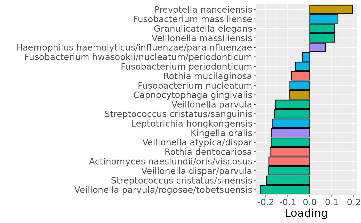
c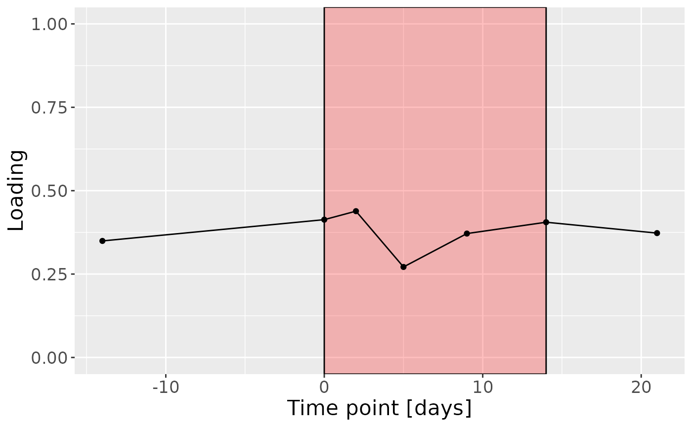
Upper jaw interproximal microbiome
CP was applied to capture the dominant source of variation in the upper jaw interproximal microbiome data block. The model selection procedure revealed that CORCONDIA scores were inconclusive and loadings were unstable at three components. The commented code below performs the procedure, and is not rerun here due to computational limitations.
# assessment_upinter = parafac4microbiome::assessModelQuality(processedUpinter$data, numRepetitions=10, numCores=10)

# assessment_upinter$metrics$CORCONDIA %>% as_tibble() %>% mutate(index=1:nrow(.)) %>% pivot_longer(-index) %>% ggplot(aes(x=as.factor(name),y=value)) + geom_boxplot() + xlab("Number of components") + ylab("CORCONDIA") + theme(text=element_text(size=16))

# stability_upinter = parafac4microbiome::assessModelStability(processedUpinter, maxNumComponents=3, numFolds=10, colourCols=colourCols, legendTitles=legendTitles, xLabels = xLabels, legendColNums=legendColNums, arrangeModes=arrangeModes, numCores=parallel::detectCores())
# stability_upinter$modelPlots[[2]]
# stability_upinter$modelPlots[[3]]
#
# cp_upinter = parafac4microbiome::parafac(processedUpinter$data, nfac=2, nstart=100)
cp_upinter = readRDS("./TIFN2/cp_upinter.RDS")

cp_upinter$varExp
## [1] 16.10052Therefore, a two-component CP model was selected, explaining 16.1% of the variation. However, MLR analysis revealed that the first CP component captured variation associated with a mixture of BOMP% and subject gender, while the second component was not interpretable.
testMetadata(cp_upinter, 1, processedUpinter)## Term Estimate CI
## 1 plaquepercent 2.1326839 -0.00328755891087678 – 0.00755292666044199
## 2 bomppercent 3.7419573 0.000355581649636956 – 0.00712833294888875
## 3 Area_delta_R30 6.3702807 -0.000458619993549555 – 0.013199181483497
## 4 gender 114.7064044 0.0185514573648732 – 0.210861351396827
## 5 age -0.6618349 -0.00922631147351948 – 0.00790264161581984
## P_value P_adjust
## 1 0.42980563 0.53725704
## 2 0.03130954 0.07827386
## 3 0.06654502 0.11090837
## 4 0.02076356 0.07827386
## 5 0.87624079 0.87624079
testMetadata(cp_upinter, 2, processedUpinter)## Term Estimate CI
## 1 plaquepercent -2.4316053 -0.00867251409160288 – 0.00380930341158905
## 2 bomppercent 2.7501722 -0.00114892641938689 – 0.00664927091740296
## 3 Area_delta_R30 -0.9668053 -0.0088296535710741 – 0.00689604288502859
## 4 gender 30.5288503 -0.0801846866985154 – 0.141242387353944
## 5 age -7.7000402 -0.0175612435880203 – 0.00216116322441363
## P_value P_adjust
## 1 0.4342843 0.7238072
## 2 0.1610410 0.4026024
## 3 0.8043410 0.8043410
## 4 0.5791848 0.7239810
## 5 0.1219174 0.4026024
testFeatures(cp_upinter, processedUpinter, 1, "bomppercent") # flip## Joining with `by = join_by(subject, RFgroup)`
## Joining with `by = join_by(subject, age, gender)`## [1] "Positive loadings:"
## bomppercent
## [1,] -0.4565796
## [1] "Negative loadings:"
## bomppercent
## [1,] 0.4565796
testFeatures(cp_upinter, processedUpinter, 1, "gender") # flip## Joining with `by = join_by(subject, RFgroup)`
## Joining with `by = join_by(subject, age, gender)`## [1] "Positive loadings:"
## gender
## [1,] -0.2166038
## [1] "Negative loadings:"
## gender
## [1,] 0.2166038
a = processedUpinter$mode1 %>%
  mutate(Component_1 = cp_upinter$Fac[[1]][,1]) %>%
  left_join(rf_data %>% select(subject,day,Area_delta_R30,plaquepercent,bomppercent) %>% filter(day==14), by="subject") %>%
  ggplot(aes(x=bomppercent,y=Component_1)) +
  geom_point() +
  xlab("BOMP%") +
  ylab("Loading") +
  stat_cor() +
  theme(text=element_text(size=16))

b = plotFeatures(processedUpinter$mode2, cp_upinter, 1, flip=TRUE) + scale_fill_manual(values=phylum_colors[-c(3,7)]) + theme(legend.position="none")

c = processedUpinter$mode3 %>%
  mutate(Component_1 = -1*cp_upinter$Fac[[3]][,1], day=c(-14,0,2,5,9,14,21)) %>%
  ggplot(aes(x=day,y=Component_1)) +
  annotate(geom = "rect", xmin = 0, xmax = 14, ymin = -Inf, ymax = Inf, fill = "red", colour = "black", alpha=0.25) +
  geom_line() +
  geom_point() +
  xlab("Time point [days]") +
  ylab("Loading") +
  ylim(0,1) +
  theme(legend.position="none", text=element_text(size=16))

a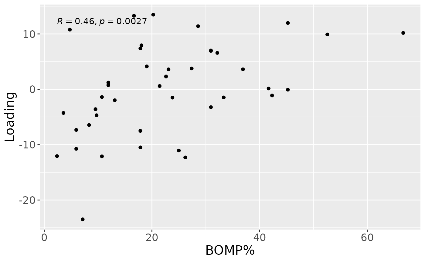
b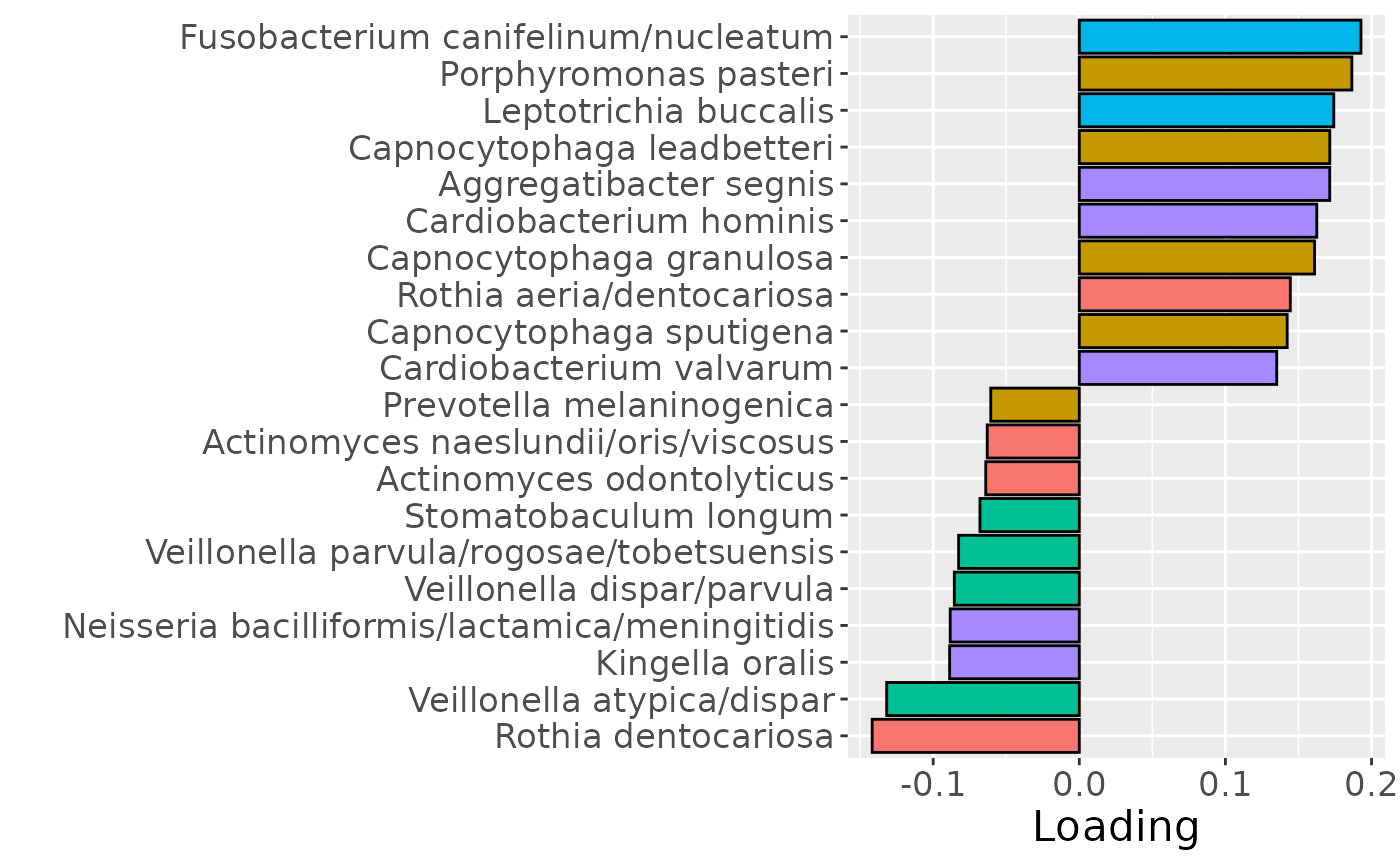
c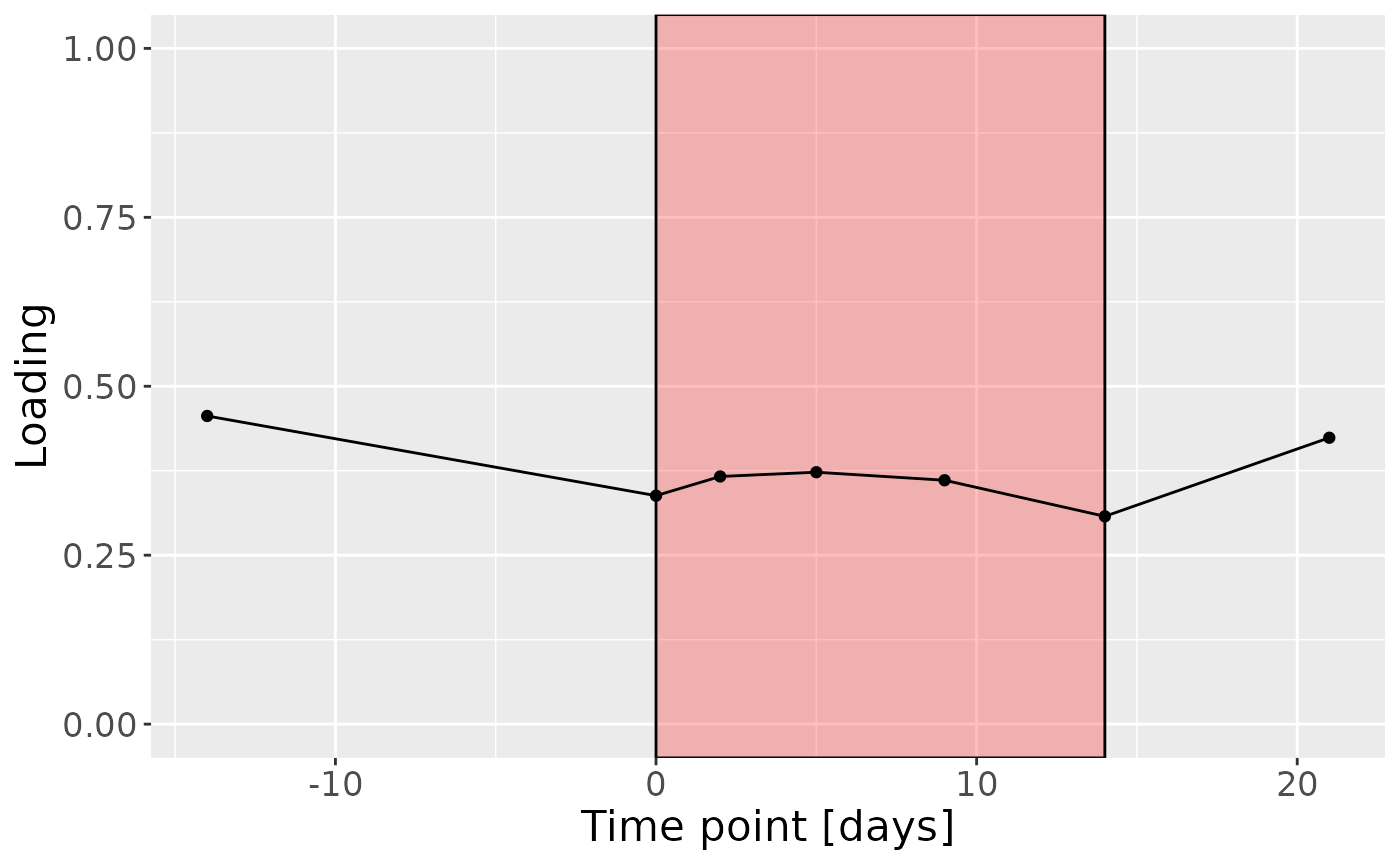
Salivary microbiome
CP was applied to capture the dominant source of variation in the salivary microbiome data block. The model selection procedure revealed that CORCONDIA scores were too low at three components. The commented code below performs the procedure, and is not rerun here due to computational limitations.
# assessment_saliva = parafac4microbiome::assessModelQuality(processedSaliva$data, numRepetitions=10, numCores=10)

# assessment_saliva$metrics$CORCONDIA %>% as_tibble() %>% mutate(index=1:nrow(.)) %>% pivot_longer(-index) %>% ggplot(aes(x=as.factor(name),y=value)) + geom_boxplot() + xlab("Number of components") + ylab("CORCONDIA") + theme(text=element_text(size=16))

# stability_saliva = parafac4microbiome::assessModelStability(processedSaliva, maxNumComponents=3, numFolds=10, colourCols=colourCols, legendTitles=legendTitles, xLabels = xLabels, legendColNums=legendColNums, arrangeModes=arrangeModes, numCores=parallel::detectCores())
# stability_saliva$modelPlots[[2]]
# stability_saliva$modelPlots[[3]]
#
# cp_saliva = parafac4microbiome::parafac(processedSaliva$data, nfac=2, nstart=100)
cp_saliva = readRDS("./TIFN2/cp_saliva.RDS")

cp_saliva$varExp
## [1] 17.33499Therefore, a two-component CP model was selected, explaining 17.3% of the variation. However, MLR analysis revealed that the first CP component captured uninterpretable variation, while the second component captured variation exclusively associated with subject age.
testMetadata(cp_saliva, 1, processedSaliva)## Term Estimate CI
## 1 plaquepercent 2.410738 -0.00355831149506644 – 0.00837978682976563
## 2 bomppercent -2.504120 -0.00623337039896853 – 0.00122513045951894
## 3 Area_delta_R30 -5.519053 -0.0130393880948642 – 0.00200128290288186
## 4 gender -86.946657 -0.192837413136006 – 0.0189440987425446
## 5 age -7.035609 -0.0164672494454233 – 0.00239603161672677
## P_value P_adjust
## 1 0.4178187 0.4178187
## 2 0.1815319 0.2269149
## 3 0.1452174 0.2269149
## 4 0.1044564 0.2269149
## 5 0.1389100 0.2269149
testMetadata(cp_saliva, 2, processedSaliva)## Term Estimate CI
## 1 plaquepercent 4.868327 -0.000666119508513777 – 0.0104027729980185
## 2 bomppercent 1.049513 -0.00240821269203614 – 0.00450723916772543
## 3 Area_delta_R30 5.576203 -0.00139658153889448 – 0.0125489871748319
## 4 gender 59.330741 -0.0388501724466451 – 0.157511653873589
## 5 age -11.908698 -0.0206536259300458 – -0.00316376911062791
## P_value P_adjust
## 1 0.08280442 0.1890952
## 2 0.54175458 0.5417546
## 3 0.11345712 0.1890952
## 4 0.22808875 0.2851109
## 5 0.00903208 0.0451604
testFeatures(cp_saliva, processedSaliva, 2, "age") # no flip## Joining with `by = join_by(subject, RFgroup)`
## Joining with `by = join_by(subject, age, gender)`## [1] "Positive loadings:"
## age
## [1,] 0.3592963
## [1] "Negative loadings:"
## age
## [1,] -0.3592963
a = processedSaliva$mode1 %>%
  mutate(Component_1 = cp_saliva$Fac[[1]][,2]) %>%
  left_join(rf_data %>% select(subject,day,Area_delta_R30,plaquepercent,bomppercent) %>% filter(day==14), by="subject") %>%
  ggplot(aes(x=age,y=Component_1)) +
  geom_point() +
  xlab("Age") +
  ylab("Loading") +
  stat_cor() +
  theme(text=element_text(size=16))

b = plotFeatures(processedSaliva$mode2, cp_saliva, 2, flip=FALSE) + scale_fill_manual(values=phylum_colors[-c(7)]) + theme(legend.position="none")

c = processedSaliva$mode3 %>%
  mutate(Component_1 = -1*cp_saliva$Fac[[3]][,2], day=c(-14,0,2,5,9,14,21)) %>%
  ggplot(aes(x=day,y=Component_1)) +
  annotate(geom = "rect", xmin = 0, xmax = 14, ymin = -Inf, ymax = Inf, fill = "red", colour = "black", alpha=0.25) +
  geom_line() +
  geom_point() +
  xlab("Time point [days]") +
  ylab("Loading") +
  ylim(0,1) +
  theme(legend.position="none", text=element_text(size=16))

a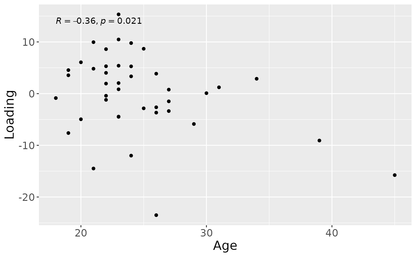
b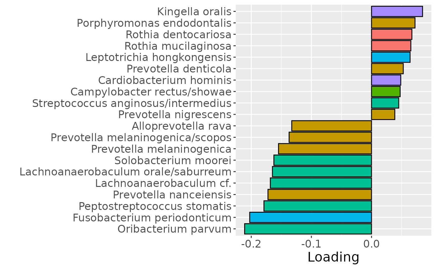
c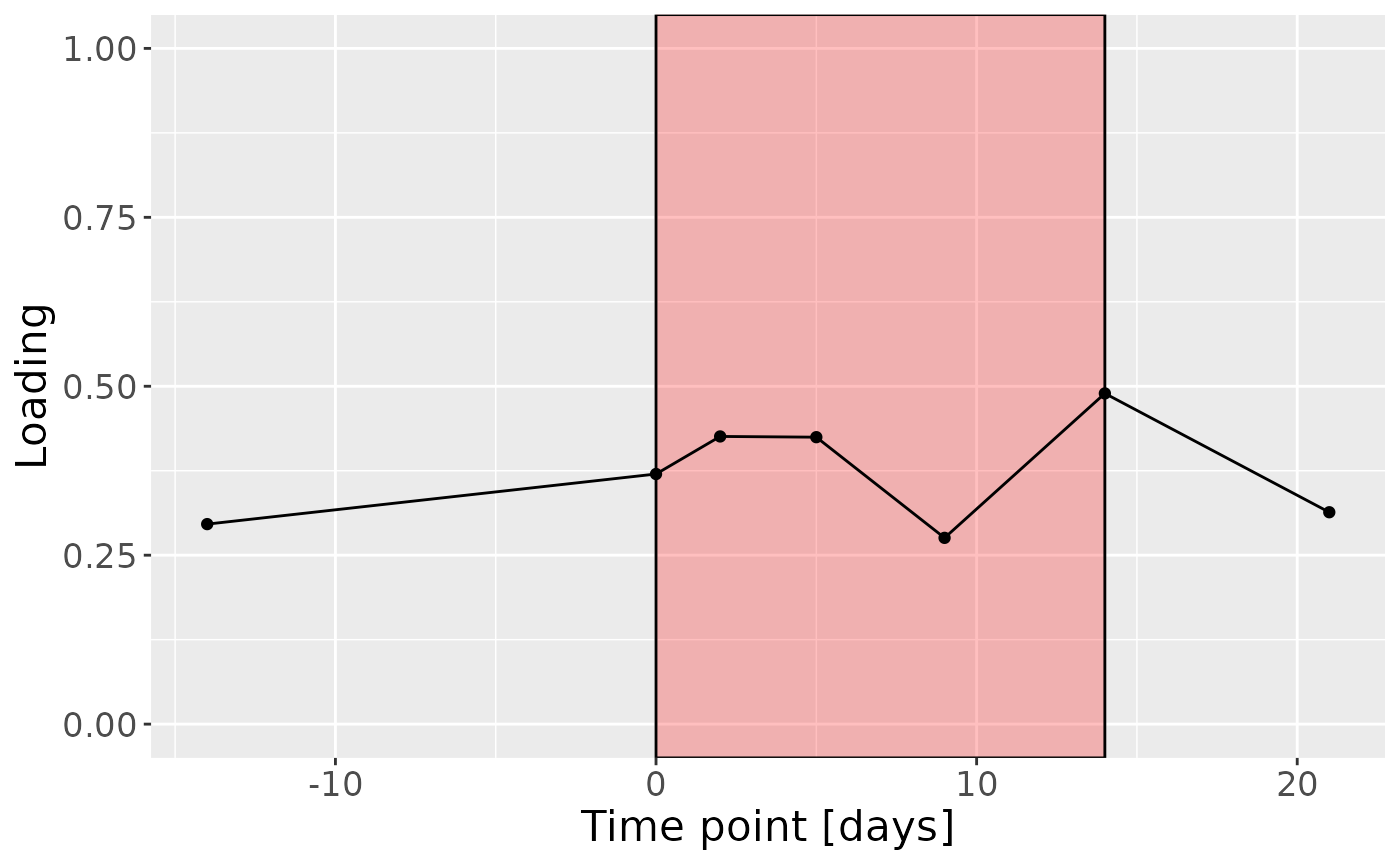
Salivary metabolomics
CP was applied to capture the dominant source of variation in the salivary metabolomics data block. The model selection procedure revealed that CORCONDIA scores were too low at two components. The commented code below performs the procedure, and is not rerun here due to computational limitations.
# assessment_metab = parafac4microbiome::assessModelQuality(processedMetabolomics$data, numRepetitions=10, numCores=10)

# assessment_metab$metrics$CORCONDIA %>% as_tibble() %>% mutate(index=1:nrow(.)) %>% pivot_longer(-index) %>% ggplot(aes(x=as.factor(name),y=value)) + geom_boxplot() + xlab("Number of components") + ylab("CORCONDIA") + theme(text=element_text(size=16))

# stability_metab = parafac4microbiome::assessModelStability(processedMetabolomics, maxNumComponents=2, numFolds=10, colourCols=colourCols, legendTitles=legendTitles, xLabels = xLabels, legendColNums=legendColNums, arrangeModes=arrangeModes, numCores=parallel::detectCores())
# stability_metab$modelPlots[[1]]
# stability_metab$modelPlots[[2]]
# cp_metabolomics = parafac4microbiome::parafac(processedMetabolomics$data, nfac=1, nstart=100)
cp_metabolomics = readRDS("./TIFN2/cp_metabolomics.RDS")

cp_metabolomics$varExp
## [1] 15.44305Therefore, a one-component CP model was selected, explaining 15.4% of the variation. However, MLR analysis revealed that the CP component captured uninterpretable variation.
testMetadata(cp_metabolomics, 1, processedMetabolomics)## Term Estimate CI
## 1 plaquepercent 4.340779 -0.00177252492396623 – 0.0104540835526603
## 2 bomppercent 1.782998 -0.00195667074036764 – 0.00552266679650121
## 3 Area_delta_R30 3.973073 -0.00357131688284603 – 0.0115174629081315
## 4 gender -35.447349 -0.141829531868009 – 0.0709348329387957
## 5 age -7.356789 -0.0168151275419762 – 0.00210155014536747
## P_value P_adjust
## 1 0.1581698 0.3954244
## 2 0.3394212 0.4242765
## 3 0.2920535 0.4242765
## 4 0.5028867 0.5028867
## 5 0.1232062 0.3954244