MAINHEALTH: intergenerational obesity transmission
2025-08-31
Source:vignettes/articles/MAINHEALTH.Rmd
MAINHEALTH.RmdIntroduction
This article presents the CP results of the MAINHEALTH dataset discussed in Chapter 5 of my dissertation.
Preamble
##
## Attaching package: 'dplyr'
## The following objects are masked from 'package:stats':
##
## filter, lag## The following objects are masked from 'package:base':
##
## intersect, setdiff, setequal, union##
## Attaching package: 'CMTFtoolbox'## The following object is masked from 'package:NPLStoolbox':
##
## npred## The following objects are masked from 'package:parafac4microbiome':
##
## fac_to_vect, reinflateFac, reinflateTensor, vect_to_fac
testMetadata = function(model, comp, metadata){
  transformedSubjectLoadings = model$Fac[[1]][,comp]
  transformedSubjectLoadings = transformedSubjectLoadings / norm(transformedSubjectLoadings, "2")

  result = lm(transformedSubjectLoadings ~ BMI + C.section + Secretor + Lewis + whz.6m, data=metadata$mode1)

  # Extract coefficients and confidence intervals
  coef_estimates <- summary(result)$coefficients
  conf_intervals <- confint(result)

  # Remove intercept
  coef_estimates <- coef_estimates[rownames(coef_estimates) != "(Intercept)", ]
  conf_intervals <- conf_intervals[rownames(conf_intervals) != "(Intercept)", ]

  # Combine into a clean data frame
  summary_table <- data.frame(
    Term     = rownames(coef_estimates),
    Estimate = coef_estimates[, "Estimate"] * 1e3,
    CI       = paste0(
                 conf_intervals[, 1], " – ",
                 conf_intervals[, 2]
               ),
    P_value  = coef_estimates[, "Pr(>|t|)"],
    P_adjust = p.adjust(coef_estimates[, "Pr(>|t|)"], "BH"),
    row.names = NULL
  )

  return(summary_table)
}
colours = RColorBrewer:: brewer.pal(8, "Dark2")
BMI_cols = c("darkgreen","darkgoldenrod","darkred") #colours[1:3]
WHZ_cols = c("darkgreen", "darkgoldenrod", "dodgerblue4")
phylum_cols = colours
processedFaeces = parafac4microbiome::processDataCube(NPLStoolbox::Jakobsen2025$faeces, sparsityThreshold = 0.75, centerMode=1, scaleMode=2)
processedMilk = parafac4microbiome::processDataCube(NPLStoolbox::Jakobsen2025$milkMicrobiome, sparsityThreshold=0.85, centerMode=1, scaleMode=2)
processedMilkMetab = parafac4microbiome::processDataCube(NPLStoolbox::Jakobsen2025$milkMetabolomics, CLR=FALSE, centerMode=1, scaleMode=2)Faecal microbiome
CP was applied to capture the dominant source of variation in the infant faecal microbiome data block. The model selection procedure revealed that CORCONDIA was inconclusive and loadings were somewhat unstable at three components. The commented code below performs the procedure, and is not rerun here due to computational limitations.
# assessment_faeces = parafac4microbiome::assessModelQuality(processedFaeces$data, numRepetitions = 10, numCores = 10)
# assessment_faeces$metrics$CORCONDIA %>% as_tibble() %>% mutate(index=1:nrow(.)) %>% pivot_longer(-index) %>% ggplot(aes(x=as.factor(name),y=value)) + geom_boxplot() + xlab("Number of components") + ylab("CORCONDIA") + theme(text=element_text(size=16))

# stability_faeces = parafac4microbiome::assessModelStability(processedFaeces, maxNumComponents=3, numFolds=20, colourCols=colourCols, legendTitles=legendTitles, xLabels = xLabels, legendColNums=legendColNums, arrangeModes=arrangeModes, numCores=parallel::detectCores())
# stability_faeces$modelPlots[[2]]
# stability_faeces$modelPlots[[3]]
#
# cp_faeces = parafac4microbiome::parafac(processedFaeces$data, nfac=3, nstart = 100)
cp_faeces = readRDS("./MAINHEALTH/cp_faeces.RDS")

cp_faeces$varExp
## [1] 15.17823Therefore, a two-component CP model was selected, explaining 15.2% of the variation. However, MLR analysis revealed that neither component could be interpreted.
testMetadata(cp_faeces, 1, processedFaeces)## Term Estimate CI P_value
## 1 BMI 1.557682 -0.00109277376368493 – 0.00420813678843941 0.24698916
## 2 C.section -17.096372 -0.0655708277484862 – 0.0313780847296313 0.48646498
## 3 Secretor 11.375601 -0.0221113148908448 – 0.0448625169392564 0.50262459
## 4 Lewis -86.360039 -0.181248173947069 – 0.00852809560447294 0.07407419
## 5 whz.6m -3.321885 -0.0160020917474101 – 0.0093583227214069 0.60504067
## P_adjust
## 1 0.6050407
## 2 0.6050407
## 3 0.6050407
## 4 0.3703709
## 5 0.6050407
testMetadata(cp_faeces, 2, processedFaeces)## Term Estimate CI P_value
## 1 BMI 2.722216 -4.56020479994157e-06 – 0.00544899180328022 0.05037851
## 2 C.section 46.004176 -0.003866118532671 – 0.0958744696412498 0.07028311
## 3 Secretor -7.108612 -0.041559794510577 – 0.027342570748067 0.68370085
## 4 Lewis -60.366832 -0.157987302185625 – 0.0372536372194021 0.22330820
## 5 whz.6m 1.450616 -0.0115947217747149 – 0.0144959541369427 0.82617195
## P_adjust
## 1 0.1757078
## 2 0.1757078
## 3 0.8261720
## 4 0.3721803
## 5 0.8261720HM microbiome
CP was applied to capture the dominant source of variation in the HM microbiome data block. The model selection procedure revealed that CORCONDIA was inconclusive and loadings were unstable at three components. The commented code below performs the procedure, and is not rerun here due to computational limitations.
# assessment_milk = parafac4microbiome::assessModelQuality(processedMilk$data, numRepetitions = 10, numCores = 10)
# assessment_milk$metrics$CORCONDIA %>% as_tibble() %>% mutate(index=1:nrow(.)) %>% pivot_longer(-index) %>% ggplot(aes(x=as.factor(name),y=value)) + geom_boxplot() + xlab("Number of components") + ylab("CORCONDIA") + theme(text=element_text(size=16))

# stability_milk = parafac4microbiome::assessModelStability(processedMilk, maxNumComponents=3, numFolds=10, colourCols=colourCols, legendTitles=legendTitles, xLabels = xLabels, legendColNums=legendColNums, arrangeModes=arrangeModes, numCores=parallel::detectCores())
# stability_milk$modelPlots[[2]]
# stability_milk$modelPlots[[3]]
#
# cp_milk = parafac4microbiome::parafac(processedMilk$data, nfac=2, nstart = 100)
cp_milk = readRDS("./MAINHEALTH/cp_milk.RDS")
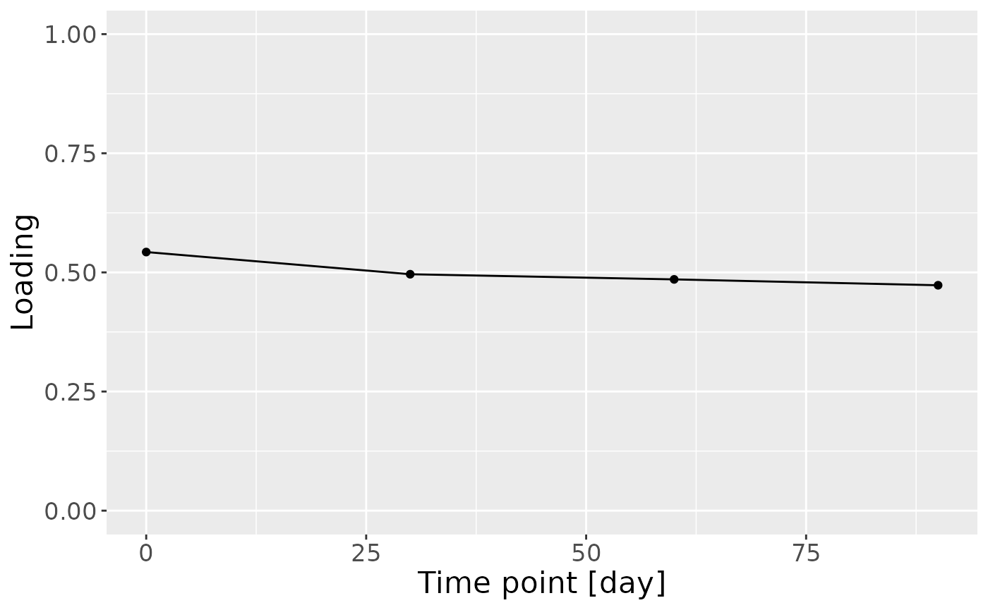
cp_milk$varExp## [1] 13.17473Therefore, a two-component CP model was selected, explaining 13.2% of the variation. However, MLR analysis revealed that the first CP component was uninterpretable, while the second captured variation only weakly associated with maternal ppBMI.
testMetadata(cp_milk, 1, processedMilk)## Term Estimate CI P_value
## 1 BMI -0.7971158 -0.00356908227805278 – 0.00197485067980183 0.5702715
## 2 C.section -27.2768492 -0.0779905182386613 – 0.0234368199177587 0.2891367
## 3 Secretor 4.8853309 -0.0301641355434441 – 0.039934797247701 0.7830997
## 4 Lewis 28.0599419 -0.071151776413022 – 0.127271660144112 0.5766273
## 5 whz.6m 2.3991703 -0.0108741423856309 – 0.015672483059881 0.7211329
## P_adjust
## 1 0.7830997
## 2 0.7830997
## 3 0.7830997
## 4 0.7830997
## 5 0.7830997
testMetadata(cp_milk, 2, processedMilk)## Term Estimate CI P_value
## 1 BMI 2.942392 0.000305899155017146 – 0.00557888463379954 0.02901701
## 2 C.section 25.569124 -0.0226660263261727 – 0.0738042746886722 0.29612537
## 3 Secretor 6.165320 -0.0271711809286324 – 0.0395018213417433 0.71494998
## 4 Lewis -74.787457 -0.169150421245261 – 0.0195755080850167 0.11927081
## 5 whz.6m -3.204212 -0.0158288212471368 – 0.00942039651018406 0.61630886
## P_adjust
## 1 0.1450850
## 2 0.4935423
## 3 0.7149500
## 4 0.2981770
## 5 0.7149500
topIndices = processedMilk$mode2 %>% mutate(index=1:nrow(.), Comp = cp_milk$Fac[[2]][,2]) %>% arrange(desc(Comp)) %>% head() %>% select(index) %>% pull()
bottomIndices = processedMilk$mode2 %>% mutate(index=1:nrow(.), Comp = cp_milk$Fac[[2]][,2]) %>% arrange(desc(Comp)) %>% tail() %>% select(index) %>% pull()

Xhat = parafac4microbiome::reinflateTensor(cp_milk$Fac[[1]][,2], cp_milk$Fac[[2]][,2], cp_milk$Fac[[3]][,2])

print("Positive loadings:")
## [1] "Positive loadings:"## [1] 0.1705408
print("Negative loadings:")## [1] "Negative loadings:"## [1] -0.1705408
a = processedMilk$mode1 %>%
  mutate(Component_2 = cp_milk$Fac[[1]][,2]) %>%
  ggplot(aes(x=BMI,y=Component_2)) +
  geom_point() +
  stat_cor() +
  xlab("ppBMI") +
  ylab("Loading") +
  theme(text=element_text(size=16))

df = processedMilk$mode2 %>%
  mutate(Component_2 = cp_milk$Fac[[2]][,2]) %>%
  arrange(Component_2) %>%
  mutate(index=1:nrow(.)) %>%
  mutate(Genus = gsub("g__", "", V7), Species = gsub("s__", "", V8)) %>%
  mutate(Species = str_split_fixed(Species, "_", 2)[,2]) %>%
  mutate(dplyr::across(.cols = Species, .fns = ~ dplyr::if_else(stringr::str_detect(.x, "sp."), "", .x))) %>%
  mutate(dplyr::across(.cols = Species, .fns = ~ dplyr::if_else(stringr::str_detect(.x, "organism"), "", .x))) %>%
  mutate(dplyr::across(.cols = Species, .fns = ~ dplyr::if_else(stringr::str_detect(.x, "bacterium"), "", .x))) %>%
  filter(index %in% c(1:10, 106:115))

df[df$Genus == "" & df$Species == "", "Species"] = "Unknown"
df[df$Species == "", "Species"] = "sp."
df$name = paste0(df$Genus, " ", df$Species)

b = df %>% ggplot(aes(x=Component_2,y=as.factor(index),fill=as.factor(V3))) +
  geom_bar(stat="identity", col="black") +
  xlab("Loading") +
  ylab("") +
  scale_y_discrete(labels=df$name) +
  scale_fill_manual(name="Phylum", values=hue_pal()(5)[-c(2,5)], labels=c("Actinobacteriota", "Firmicutes", "Proteobacteria")) +
  theme(text=element_text(size=16))

c = cp_milk$Fac[[3]][,2] %>%
  as_tibble() %>%
  mutate(value=value) %>%
  ggplot(aes(x=c(0,30,60,90),y=value)) +
  geom_line() +
  geom_point() +
  xlab("Time point [day]") +
  ylab("Loading") +
  ylim(0,1) +
  theme(text=element_text(size=16))

a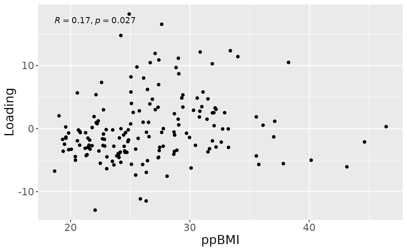
b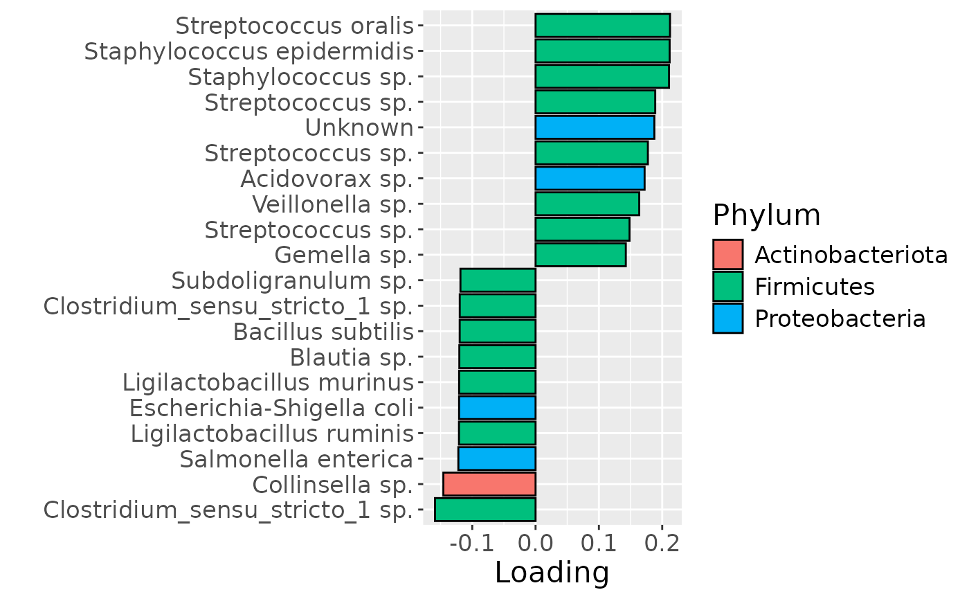
c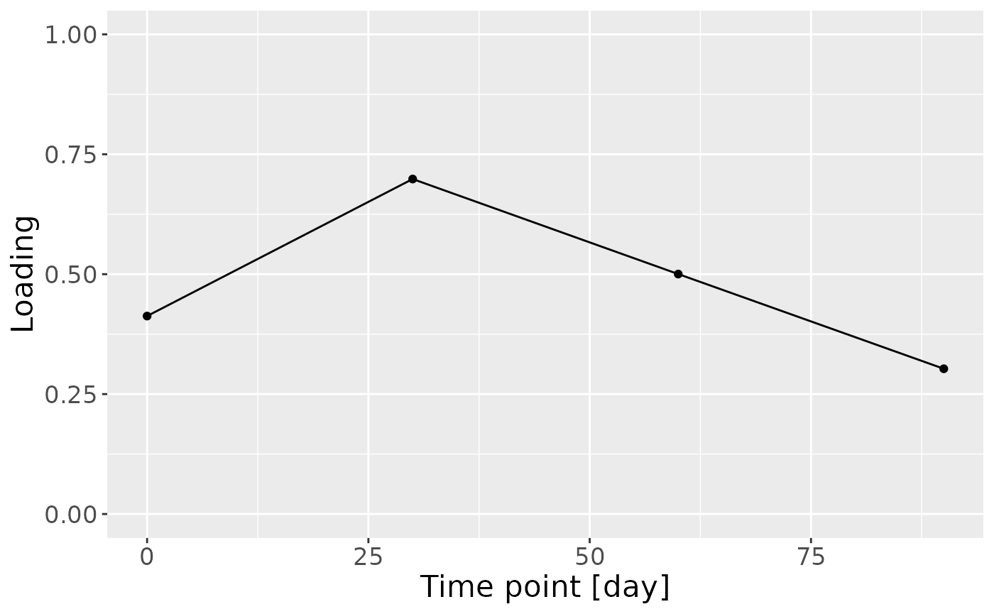
HM metabolome
CP was applied to capture the dominant source of variation in the HM metabolomics data block. The model selection procedure revealed that CORCONDIA values were too low at four components. The commented code below performs the procedure, and is not rerun here due to computational limitations.
# assessment_milkMetab = parafac4microbiome::assessModelQuality(processedMilkMetab$data, numRepetitions = 10, numCores = 10)
#
# assessment_milkMetab$metrics$CORCONDIA %>% as_tibble() %>% mutate(index=1:nrow(.)) %>% pivot_longer(-index) %>% ggplot(aes(x=as.factor(name),y=value)) + geom_boxplot() + xlab("Number of components") + ylab("CORCONDIA") + theme(text=element_text(size=16))

# stability_milkMetab = parafac4microbiome::assessModelStability(processedMilkMetab, maxNumComponents=4, numFolds=10, colourCols=c("", "", ""), legendTitles=c("BMI group", "Class", ""), xLabels = xLabels, legendColNums=legendColNums, arrangeModes=arrangeModes, numCores=parallel::detectCores())
# stability_milkMetab$modelPlots[[3]]
# stability_milkMetab$modelPlots[[4]]
# cp_milkMetab = parafac4microbiome::parafac(processedMilkMetab$data, nfac=3, nstart = 100)
cp_milkMetab = readRDS("./MAINHEALTH/cp_milkMetab.RDS")

cp_milkMetab$varExp
## [1] 21.55482Therefore, a three-component CP model was selected, explaining 21.6% of the variation. MLR analysis revealed that the first and third components were uninterpretable, while the second component captured variation exclusively and strongly associated with maternal secretor status.
testMetadata(cp_milkMetab, 1, processedMilkMetab)## Term Estimate CI P_value
## 1 BMI -2.583661 -0.00535718628987143 – 0.000189863674592802 0.06760372
## 2 C.section -9.956381 -0.0605921878622612 – 0.0406794268355845 0.69782750
## 3 Secretor 9.252236 -0.0261442697993304 – 0.0446487419625543 0.60584696
## 4 Lewis 92.519158 -0.0281341347345387 – 0.213172450952438 0.13163311
## 5 whz.6m 10.497357 -0.00275014531882957 – 0.0237448598441314 0.11934771
## P_adjust
## 1 0.2193885
## 2 0.6978275
## 3 0.6978275
## 4 0.2193885
## 5 0.2193885
testMetadata(cp_milkMetab, 2, processedMilkMetab)## Term Estimate CI P_value
## 1 BMI 0.1116855 -0.00080493346242961 – 0.0010283045137446 8.098366e-01
## 2 C.section 11.0721065 -0.00566246154228743 – 0.0278066745141615 1.927839e-01
## 3 Secretor 177.1666463 0.165468496949462 – 0.188864795602086 6.443800e-59
## 4 Lewis -37.4429441 -0.0773175080477337 – 0.00243161979792261 6.545970e-02
## 5 whz.6m 1.6165731 -0.0027615783945977 – 0.00599472449699943 4.662904e-01
## P_adjust
## 1 8.098366e-01
## 2 3.213065e-01
## 3 3.221900e-58
## 4 1.636492e-01
## 5 5.828630e-01
testMetadata(cp_milkMetab, 3, processedMilkMetab)## Term Estimate CI P_value
## 1 BMI -1.716400 -0.00415552494908338 – 0.000722724998462952 0.1661829
## 2 C.section -22.466123 -0.0669968421278869 – 0.0220645963398689 0.3199733
## 3 Secretor -6.672137 -0.0378009361212165 – 0.0244566617238421 0.6721456
## 4 Lewis -22.466704 -0.128572999236914 – 0.0836395906101599 0.6758950
## 5 whz.6m 3.066525 -0.00858374497479842 – 0.0147167946587828 0.6033337
## P_adjust
## 1 0.675895
## 2 0.675895
## 3 0.675895
## 4 0.675895
## 5 0.675895
topIndices = processedMilkMetab$mode2 %>% mutate(index=1:nrow(.), Comp = cp_milkMetab$Fac[[2]][,2]) %>% arrange(desc(Comp)) %>% head() %>% select(index) %>% pull()
bottomIndices = processedMilkMetab$mode2 %>% mutate(index=1:nrow(.), Comp = cp_milkMetab$Fac[[2]][,2]) %>% arrange(desc(Comp)) %>% tail() %>% select(index) %>% pull()

Xhat = parafac4microbiome::reinflateTensor(cp_milkMetab$Fac[[1]][,2], cp_milkMetab$Fac[[2]][,2], cp_milkMetab$Fac[[3]][,2])

print("Positive loadings:")
## [1] "Positive loadings:"## [1] -0.9257706
print("Negative loadings:")## [1] "Negative loadings:"## [1] 0.9257706
a = processedMilkMetab$mode1 %>%
  mutate(Component_2 = cp_milkMetab$Fac[[1]][,2]) %>%
  ggplot(aes(x=as.factor(Secretor),y=Component_2)) +
  geom_boxplot() +
  stat_compare_means() +
  xlab("Secretor status") +
  ylab("Loading") +
  scale_x_discrete(labels=c("Se-", "Se+")) +
  theme(text=element_text(size=16))

temp = processedMilkMetab$mode2 %>%
  mutate(Component_2 = -1*cp_milkMetab$Fac[[2]][,2]) %>%
  arrange(Component_2) %>%
  mutate(index=1:nrow(.)) %>%
  filter(index %in% c(1:10, 61:70))

b=temp %>%
  ggplot(aes(x=Component_2,y=as.factor(index),fill=as.factor(Class),pattern=as.factor(Class))) +
  geom_bar_pattern(stat="identity",
                   colour="black",
                   pattern="stripe",
                   pattern_fill="black",
                   pattern_density=0.2,
                   pattern_spacing=0.05,
                   pattern_angle=45,
                   pattern_size=0.2) +
  scale_y_discrete(label=temp$Metabolite) +
  xlab("Loading") +
  ylab("") +
  scale_fill_manual(name="Class", values=hue_pal()(7)[-c(4,5)], labels=c("Amino acids and derivatives", "Energy related", "Fatty acids and derivatives", "Oligosaccharides", "Sugars")) +
  theme(text=element_text(size=16))

c = cp_milkMetab$Fac[[3]][,2] %>%
  as_tibble() %>%
  mutate(value=value*-1) %>%
  ggplot(aes(x=c(0,30,60,90),y=value)) +
  geom_line() +
  geom_point() +
  xlab("Time point [day]") +
  ylab("Loading") +
  ylim(0,1) +
  theme(text=element_text(size=16))

a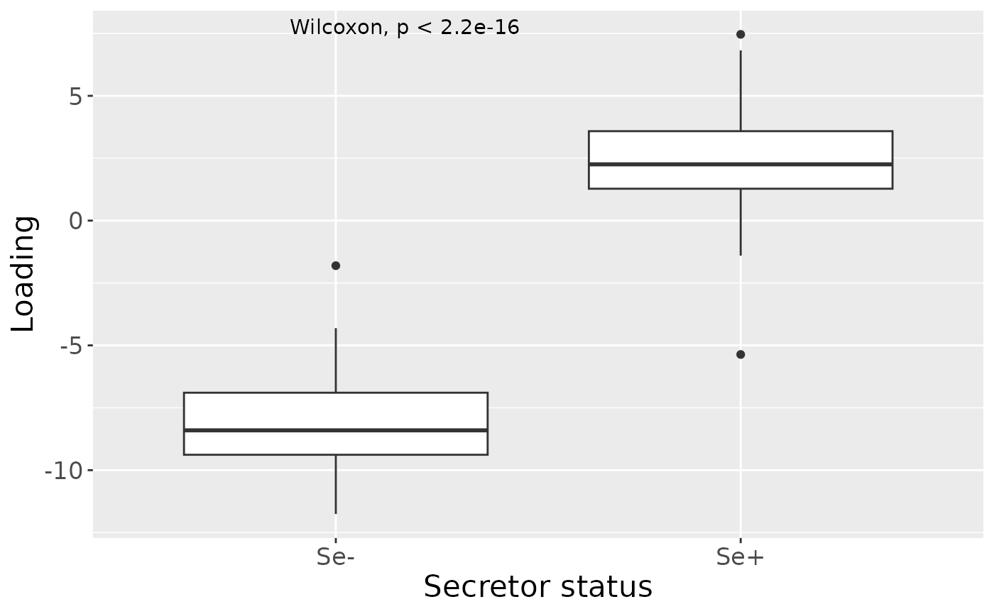
b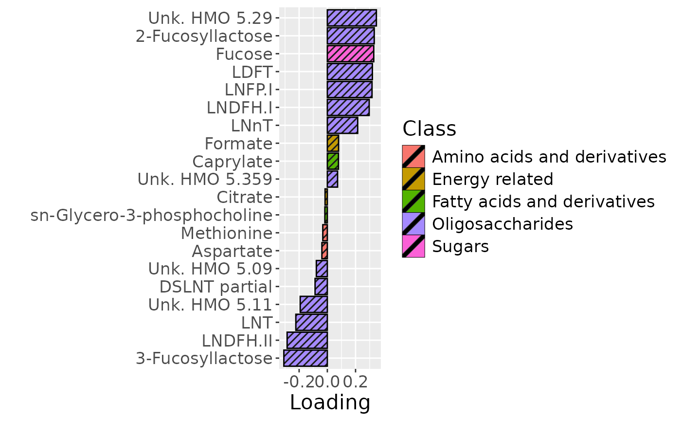
c