Preamble
library(dplyr)
#>
#> Attaching package: 'dplyr'
#> The following objects are masked from 'package:stats':
#>
#>     filter, lag
#> The following objects are masked from 'package:base':
#>
#>     intersect, setdiff, setequal, union
library(tidyr)
library(parafac4microbiome)
library(NPLStoolbox)
library(CMTFtoolbox)
#>
#> Attaching package: 'CMTFtoolbox'
#> The following object is masked from 'package:NPLStoolbox':
#>
#>     npred
#> The following objects are masked from 'package:parafac4microbiome':
#>
#>     fac_to_vect, reinflateFac, reinflateTensor, vect_to_fac
library(ggplot2)
library(ggpubr)
library(scales)
library(stringr)
testMetadata = function(model, comp, metadata){

  transformedSubjectLoadings = model$Fac[[1]][,comp]
  transformedSubjectLoadings = transformedSubjectLoadings / norm(transformedSubjectLoadings, "2")

  metadata = metadata$mode1 %>% left_join(ageInfo, by="SubjectID") %>% mutate(Gender=as.numeric(as.factor(Gender), PainS_NopainA=as.numeric(as.factor(PainS_NopainA))))
  result = lm(transformedSubjectLoadings ~ Gender + Age + PainS_NopainA, data=metadata)

  # Extract coefficients and confidence intervals
  coef_estimates <- summary(result)$coefficients
  conf_intervals <- confint(result)

  # Remove intercept
  coef_estimates <- coef_estimates[rownames(coef_estimates) != "(Intercept)", ]
  conf_intervals <- conf_intervals[rownames(conf_intervals) != "(Intercept)", ]

  # Combine into a clean data frame
  summary_table <- data.frame(
    Term     = rownames(coef_estimates),
    Estimate = coef_estimates[, "Estimate"] * 1e3,
    CI       = paste0(
                 conf_intervals[, 1], " – ",
                 conf_intervals[, 2]
               ),
    P_value  = coef_estimates[, "Pr(>|t|)"],
    P_adjust = p.adjust(coef_estimates[, "Pr(>|t|)"], "BH"),
    row.names = NULL
  )

  return(summary_table)
}ACMTF
Processing
# Microbiome
processedMicrobiome = CMTFtoolbox::Georgiou2025$Tooth_microbiome

# Remove samples due to low library size
mask = rowSums(processedMicrobiome$data) > 6500
processedMicrobiome$data = processedMicrobiome$data[mask,]
processedMicrobiome$mode1 = processedMicrobiome$mode1[mask,]

# Remove duplicate samples
mask = !(processedMicrobiome$mode1$SampleID %in% c("A11-8 36", "A11-10 17", "A11-15 17"))
processedMicrobiome$data = processedMicrobiome$data[mask,]
processedMicrobiome$mode1 = processedMicrobiome$mode1[mask,]

# Also remove subject A11-8 due to being an outlier
processedMicrobiome$data = processedMicrobiome$data[-23,,]
processedMicrobiome$mode1 = processedMicrobiome$mode1[-23,]

# CLR transformation
df = processedMicrobiome$data + 1
geomeans = pracma::geomean(as.matrix(df), dim=2)
df_clr = log(sweep(df, 1, geomeans, FUN="/"))

# Feature filtering
sparsityThreshold = 0.5
maskA = processedMicrobiome$mode1$PainS_NopainA == "A"
maskS = processedMicrobiome$mode1$PainS_NopainA == "S"

dfA = processedMicrobiome$data[maskA,]
dfS = processedMicrobiome$data[maskS,]

sparsityA = colSums(dfA == 0) / nrow(dfA)
sparsityS = colSums(dfS == 0) / nrow(dfS)

mask = (sparsityA <= sparsityThreshold) | (sparsityS <= sparsityThreshold)

processedMicrobiome$data = df_clr[,mask]
processedMicrobiome$mode2 = processedMicrobiome$mode2[mask,]

# Center and scale
processedMicrobiome$data = sweep(processedMicrobiome$data, 2, colMeans(processedMicrobiome$data), FUN="-")
processedMicrobiome$data = sweep(processedMicrobiome$data, 2, apply(processedMicrobiome$data, 2, sd), FUN="/")

# Cytokines
processedCytokines_case = CMTFtoolbox::Georgiou2025$Inflammatory_mediators

# Select only case subjects
mask = processedCytokines_case$mode1$case_control == "case"
processedCytokines_case$data = processedCytokines_case$data[mask,,]
processedCytokines_case$mode1 = processedCytokines_case$mode1[mask,]

# Select only samples with corresponding microbiome data
mask = processedCytokines_case$mode1$SubjectID %in% processedMicrobiome$mode1$SubjectID
processedCytokines_case$data = processedCytokines_case$data[mask,,]
processedCytokines_case$mode1 = processedCytokines_case$mode1[mask,]

processedCytokines_case$data = log(processedCytokines_case$data + 0.005)
processedCytokines_case$data = multiwayCenter(processedCytokines_case$data, 1)
processedCytokines_case$data = multiwayScale(processedCytokines_case$data, 2)

# Prep data
datasets = list(processedCytokines_case$data, as.matrix(processedMicrobiome$data))
modes = list(c(1,2,3),c(1,4))
Z = setupCMTFdata(datasets, modes, normalize=TRUE)
Model selection
# Please see the separate R scripts at https://doi.org/10.5281/zenodo.16993009 for the model selection.
acmtf_model = readRDS("./AP/acmtf_model.RDS")
acmtf_model$varExp
#> [1] 20.52755 27.41829
Description
ACMTF was applied to capture the dominant source of variation across the longitudinally measured inflammatory mediator and cross-sectional tooth microbiome blocks. The model selection procedure indicated that three components yielded FMS CV < 0.9. Therefore, a two-component model was selected, explaining 20.5% and 27.4% of the variation in the inflammatory mediator and tooth microbiome data blocks, respectively. The Lambda-matrix of the model revealed that the first component was predominantly distinct to the tooth microbiome block, while the second component was predominantly distinct to the inflammatory mediator block. However, MLR analysis revealed that the first component captured variation associated with a mixture of gender, age and pain perception, while the second component captured variation exclusively associated with age.
testMetadata(acmtf_model, 1, processedCytokines_case)
#>             Term    Estimate                                        CI
#> 1         Gender -149.940307   -0.25535437485488 – -0.0445262394204995
#> 2            Age    5.722737 0.00215228707320942 – 0.00929318627499447
#> 3 PainS_NopainAS -248.309324   -0.354751990816222 – -0.141866656819693
#>        P_value     P_adjust
#> 1 0.0077442196 0.0077442196
#> 2 0.0033282605 0.0049923907
#> 3 0.0001033877 0.0003101631
testMetadata(acmtf_model, 2, processedCytokines_case)
#>             Term    Estimate                                         CI
#> 1         Gender   74.084420      -0.072295300642858 – 0.22046414000031
#> 2            Age   -9.252744 -0.0142107298938554 – -0.00429475899321387
#> 3 PainS_NopainAS -102.952690    -0.250760740295701 – 0.0448553603426137
#>       P_value    P_adjust
#> 1 0.302743519 0.302743519
#> 2 0.000949563 0.002848689
#> 3 0.161212681 0.241819021
lambda = abs(acmtf_model$Fac[[5]])
colnames(lambda) = paste0("C", 1:2)

lambda %>%
  as_tibble() %>%
  mutate(block=c("cytokines", "microbiome")) %>%
  mutate(block=factor(block, levels=c("cytokines", "microbiome"))) %>%
  pivot_longer(-block) %>%
  ggplot(aes(x=as.factor(name),y=value,fill=as.factor(block))) +
  geom_bar(stat="identity",position=position_dodge(),col="black") +
  xlab("ACMTF component number") +
  ylab(expression(lambda)) +
  scale_x_discrete(labels=1:3) +
  scale_fill_manual(name="Dataset",values = hue_pal()(2),labels=c("Inflammatory mediators", "Tooth microbiome")) +
  theme(legend.position="top", text=element_text(size=16))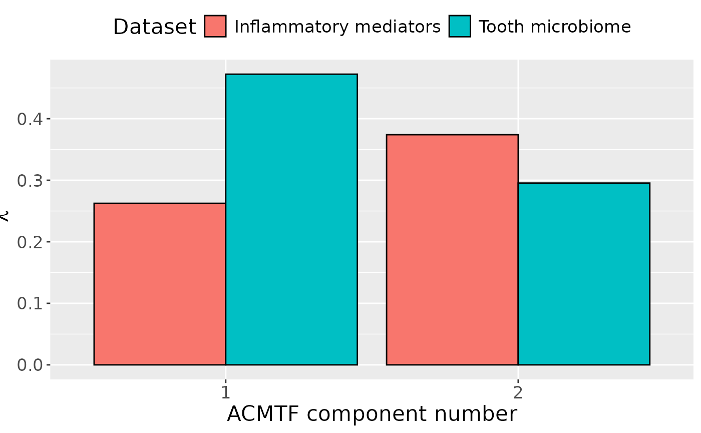
# Component 1 - gender, age, symptoms
## Cytokines
topIndices = processedCytokines_case$mode2 %>% mutate(index=1:nrow(.), Comp = acmtf_model$Fac[[2]][,1]) %>% arrange(desc(Comp)) %>% head() %>% select(index) %>% pull()
bottomIndices = processedCytokines_case$mode2 %>% mutate(index=1:nrow(.), Comp = acmtf_model$Fac[[2]][,1]) %>% arrange(desc(Comp)) %>% tail() %>% select(index) %>% pull()

Xhat = parafac4microbiome::reinflateTensor(acmtf_model$Fac[[1]][,1], acmtf_model$Fac[[2]][,1], acmtf_model$Fac[[3]][,1])

print("Positive loadings:")
#> [1] "Positive loadings:"
print(cor(Xhat[,topIndices[1],2], as.numeric(as.factor(processedCytokines_case$mode1$PainS_NopainA)), use="pairwise.complete.obs")) # flip
#> [1] -0.657178
print("Negative loadings:")
#> [1] "Negative loadings:"
print(cor(Xhat[,bottomIndices[6],2], as.numeric(as.factor(processedCytokines_case$mode1$PainS_NopainA)), use="pairwise.complete.obs"))
#> [1] 0.657178

print("Positive loadings:")
#> [1] "Positive loadings:"
print(cor(Xhat[,topIndices[1],2], processedCytokines_case$mode1 %>% left_join(ageInfo) %>% select(Age) %>% pull(), use="pairwise.complete.obs")) # no flip
#> Joining with `by = join_by(SubjectID)`
#> [1] 0.5267383
print("Negative loadings:")
#> [1] "Negative loadings:"
print(cor(Xhat[,bottomIndices[6],2], processedCytokines_case$mode1 %>% left_join(ageInfo) %>% select(Age) %>% pull(), use="pairwise.complete.obs"))
#> Joining with `by = join_by(SubjectID)`
#> [1] -0.5267383

print("Positive loadings:")
#> [1] "Positive loadings:"
print(cor(Xhat[,topIndices[1],2], as.numeric(as.factor(processedCytokines_case$mode1$Gender)), use="pairwise.complete.obs")) # flip
#> [1] -0.3425585
print("Negative loadings:")
#> [1] "Negative loadings:"
print(cor(Xhat[,bottomIndices[6],2], as.numeric(as.factor(processedCytokines_case$mode1$Gender)), use="pairwise.complete.obs"))
#> [1] 0.3425585

## Microbiome
topIndices = processedMicrobiome$mode2 %>% mutate(index=1:nrow(.), Comp = acmtf_model$Fac[[4]][,1]) %>% arrange(desc(Comp)) %>% head() %>% select(index) %>% pull()
bottomIndices = processedMicrobiome$mode2 %>% mutate(index=1:nrow(.), Comp = acmtf_model$Fac[[4]][,1]) %>% arrange(desc(Comp)) %>% tail() %>% select(index) %>% pull()

Xhat = CMTFtoolbox::reinflateMatrix(acmtf_model$Fac[[1]][,1], acmtf_model$Fac[[4]][,1])

print("Positive loadings:")
#> [1] "Positive loadings:"
print(cor(Xhat[,topIndices[1]], as.numeric(as.factor(processedCytokines_case$mode1$PainS_NopainA)), use="pairwise.complete.obs")) # flip
#> [1] -0.657178
print("Negative loadings:")
#> [1] "Negative loadings:"
print(cor(Xhat[,bottomIndices[6]], as.numeric(as.factor(processedCytokines_case$mode1$PainS_NopainA)), use="pairwise.complete.obs"))
#> [1] 0.657178

print("Positive loadings:")
#> [1] "Positive loadings:"
print(cor(Xhat[,topIndices[1]], processedCytokines_case$mode1 %>% left_join(ageInfo) %>% select(Age) %>% pull(), use="pairwise.complete.obs")) # no flip
#> Joining with `by = join_by(SubjectID)`
#> [1] 0.5267383
print("Negative loadings:")
#> [1] "Negative loadings:"
print(cor(Xhat[,bottomIndices[6]], processedCytokines_case$mode1 %>% left_join(ageInfo) %>% select(Age) %>% pull(), use="pairwise.complete.obs"))
#> Joining with `by = join_by(SubjectID)`
#> [1] -0.5267383

print("Positive loadings:")
#> [1] "Positive loadings:"
print(cor(Xhat[,topIndices[1]], as.numeric(as.factor(processedCytokines_case$mode1$Gender)), use="pairwise.complete.obs")) # flip
#> [1] -0.3425585
print("Negative loadings:")
#> [1] "Negative loadings:"
print(cor(Xhat[,bottomIndices[6]], as.numeric(as.factor(processedCytokines_case$mode1$Gender)), use="pairwise.complete.obs"))
#> [1] 0.3425585

# Component 2 - age only

## Cytokines
topIndices = processedCytokines_case$mode2 %>% mutate(index=1:nrow(.), Comp = acmtf_model$Fac[[2]][,2]) %>% arrange(desc(Comp)) %>% head() %>% select(index) %>% pull()
bottomIndices = processedCytokines_case$mode2 %>% mutate(index=1:nrow(.), Comp = acmtf_model$Fac[[2]][,2]) %>% arrange(desc(Comp)) %>% tail() %>% select(index) %>% pull()

Xhat = parafac4microbiome::reinflateTensor(acmtf_model$Fac[[1]][,2], acmtf_model$Fac[[2]][,2], acmtf_model$Fac[[3]][,2])

print("Positive loadings:")
#> [1] "Positive loadings:"
print(cor(Xhat[,topIndices[1],2], processedCytokines_case$mode1 %>% left_join(ageInfo) %>% select(Age) %>% pull(), use="pairwise.complete.obs")) # flip
#> Joining with `by = join_by(SubjectID)`
#> [1] -0.6184676
print("Negative loadings:")
#> [1] "Negative loadings:"
print(cor(Xhat[,bottomIndices[6],2], processedCytokines_case$mode1 %>% left_join(ageInfo) %>% select(Age) %>% pull(), use="pairwise.complete.obs"))
#> Joining with `by = join_by(SubjectID)`
#> [1] 0.6184676

## Microbiome
topIndices = processedMicrobiome$mode2 %>% mutate(index=1:nrow(.), Comp = acmtf_model$Fac[[4]][,2]) %>% arrange(desc(Comp)) %>% head() %>% select(index) %>% pull()
bottomIndices = processedMicrobiome$mode2 %>% mutate(index=1:nrow(.), Comp = acmtf_model$Fac[[4]][,2]) %>% arrange(desc(Comp)) %>% tail() %>% select(index) %>% pull()

Xhat = CMTFtoolbox::reinflateMatrix(acmtf_model$Fac[[1]][,2], acmtf_model$Fac[[4]][,2])

print("Positive loadings:")
#> [1] "Positive loadings:"
print(cor(Xhat[,topIndices[1]], processedCytokines_case$mode1 %>% left_join(ageInfo) %>% select(Age) %>% pull(), use="pairwise.complete.obs")) # flip
#> Joining with `by = join_by(SubjectID)`
#> [1] -0.6184676
print("Negative loadings:")
#> [1] "Negative loadings:"
print(cor(Xhat[,bottomIndices[6]], processedCytokines_case$mode1 %>% left_join(ageInfo) %>% select(Age) %>% pull(), use="pairwise.complete.obs"))
#> Joining with `by = join_by(SubjectID)`
#> [1] 0.6184676
a = processedCytokines_case$mode1 %>%
  mutate(Comp1 = acmtf_model$Fac[[1]][,1]) %>%
  ggplot(aes(x=as.factor(PainS_NopainA),y=Comp1)) +
  geom_boxplot() +
  geom_jitter(height=0, width=0.05) +
  stat_compare_means(comparisons=list(c("A", "S")),label="p.signif") +
  xlab("") +
  ylab("Loading") +
  scale_x_discrete(labels=c("Asymptomatic", "Symptomatic")) +
  theme(text=element_text(size=16))

temp = processedCytokines_case$mode2 %>%
  as_tibble() %>%
  mutate(Component_1 = -1*acmtf_model$Fac[[2]][,1]) %>%
  arrange(Component_1) %>%
  mutate(index=1:nrow(.))

b=temp %>%
  ggplot(aes(x=as.factor(index),y=Component_1)) +
  geom_bar(stat="identity",col="black") +
  scale_x_discrete(label=temp$name) +
  xlab("") +
  ylab("Loading") +
  scale_x_discrete(labels=c("OPG", "IL-4", "IL-6", expression(IL-1*beta), "IL-10", "IL-12p70", "VEGF", expression(IL-1*alpha), "IL-17A", "IL-8", expression(IFN-gamma), "GM-CSF", expression(TNF-alpha), "CRP", expression(MIP-1*alpha), "RANKL")) +
  theme(text=element_text(size=16),axis.text.x = element_text(angle = 90, vjust = 0.5, hjust=1))
#> Scale for x is already present.
#> Adding another scale for x, which will replace the existing scale.

c=acmtf_model$Fac[[3]][,1] %>%
  as_tibble() %>%
  mutate(value=value) %>%
  mutate(timepoint=c(-6,-3,0,1,6,13)) %>%
  ggplot(aes(x=timepoint,y=value)) +
  geom_line() +
  geom_point() +
  xlab("Time point [weeks]") +
  ylab("Loading") +
  ylim(0,1) +
  theme(text=element_text(size=16))

temp = processedMicrobiome$mode2 %>%
  mutate(comp=-1*acmtf_model$Fac[[4]][,1]) %>%
  mutate(Phylum = as.factor(str_split_fixed(Phylum, "__", 2)[,2]),
         Genus = str_split_fixed(Genus,"g__",2)[,2],
         Species = str_split_fixed(Species,"s__",2)[,2]) %>%
  arrange(comp) %>%
  mutate(index=1:nrow(.)) %>%
  filter(index %in% c(1:10, 143:152))

temp[temp$Species == "","Species"] = "sp."
temp[grepl("taxon", temp$Species), "Species"] = "sp."
temp$name = paste0(temp$Genus, " ", temp$Species)
temp[temp$name == " sp.","name"] = "Unknown"

d = temp %>%
  ggplot(aes(x=comp,y=as.factor(index),fill=Phylum)) +
  geom_bar(stat="identity", col="black") +
  scale_y_discrete(label=temp$name) +
  xlab("Loading") +
  ylab("") +
  scale_fill_manual(name="Phylum", labels=c("Actinobacteria", "Firmicutes", "Fusobacteria"), values=hue_pal()(6)[c(1,3,4)]) +
  theme(legend.position="none", text=element_text(size=10), axis.text.y=element_text(size=10,face="italic"))

a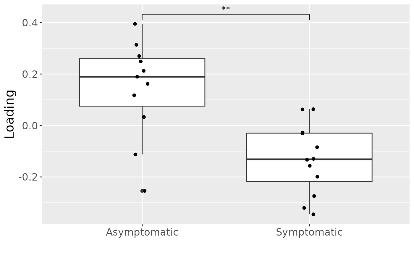
b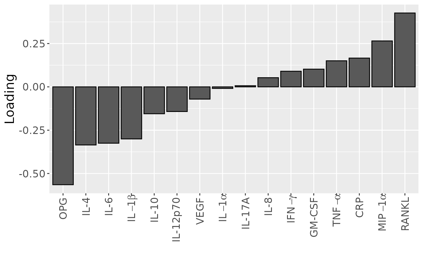
c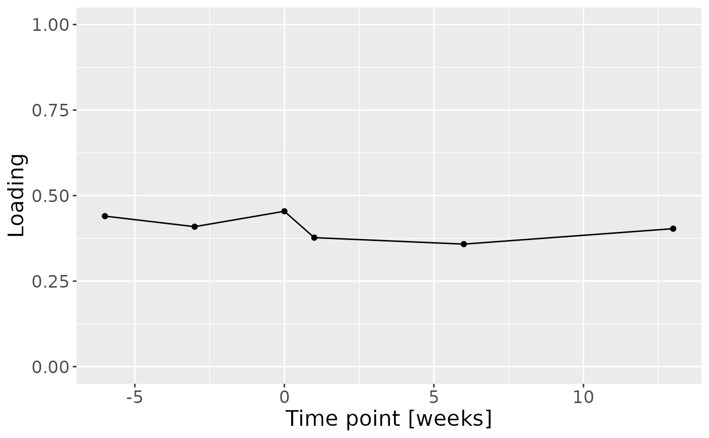
d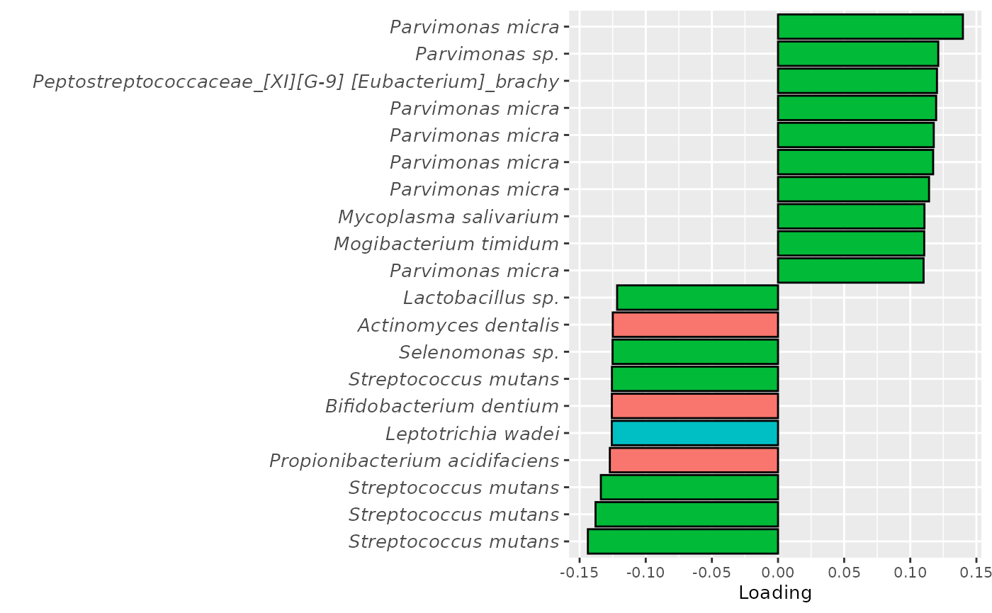
a = processedCytokines_case$mode1 %>%
  left_join(ageInfo) %>%
  mutate(Comp1 = acmtf_model$Fac[[1]][,2]) %>%
  ggplot(aes(x=Age,y=Comp1)) +
  geom_point() +
  stat_cor() +
  xlab("Age") +
  ylab("Loading") +
  theme(text=element_text(size=16))
#> Joining with `by = join_by(SubjectID)`

temp = processedCytokines_case$mode2 %>%
  as_tibble() %>%
  mutate(Component_1 = -1*acmtf_model$Fac[[2]][,2]) %>%
  arrange(Component_1) %>%
  mutate(index=1:nrow(.))

b=temp %>%
  ggplot(aes(x=as.factor(index),y=Component_1)) +
  geom_bar(stat="identity",col="black") +
  scale_x_discrete(label=temp$name) +
  xlab("") +
  ylab("Loading") +
  scale_x_discrete(labels=c("RANKL", "IL-10", "IL-6", "IL-12p70", "GM-CSF", "IL-17A", "IL-4", expression(IL-1*beta), expression(IFN-gamma), expression(IL-1*alpha), "OPG", expression(TNF-alpha), "CRP", "VEGF", expression(MIP-1*alpha), "IL-8" )) +
  theme(text=element_text(size=16),axis.text.x = element_text(angle = 90, vjust = 0.5, hjust=1))
#> Scale for x is already present.
#> Adding another scale for x, which will replace the existing scale.

c=acmtf_model$Fac[[3]][,2] %>%
  as_tibble() %>%
  mutate(value=value) %>%
  mutate(timepoint=c(-6,-3,0,1,6,13)) %>%
  ggplot(aes(x=timepoint,y=value)) +
  geom_line() +
  geom_point() +
  xlab("Time point [weeks]") +
  ylab("Loading") +
  ylim(0,1) +
  theme(text=element_text(size=16))

temp = processedMicrobiome$mode2 %>%
  mutate(comp=-1*acmtf_model$Fac[[4]][,2]) %>%
  mutate(Phylum = as.factor(str_split_fixed(Phylum, "__", 2)[,2]),
         Genus = str_split_fixed(Genus,"g__",2)[,2],
         Species = str_split_fixed(Species,"s__",2)[,2]) %>%
  arrange(comp) %>%
  mutate(index=1:nrow(.)) %>%
  filter(index %in% c(1:10, 143:152))

temp[temp$Species == "","Species"] = "sp."
temp[grepl("taxon", temp$Species), "Species"] = "sp."
temp$name = paste0(temp$Genus, " ", temp$Species)
temp[temp$name == " sp.","name"] = "Unknown"

d = temp %>%
  ggplot(aes(x=comp,y=as.factor(index),fill=Phylum)) +
  geom_bar(stat="identity", col="black") +
  scale_y_discrete(label=temp$name) +
  xlab("Loading") +
  ylab("") +
  theme(legend.position="none", text=element_text(size=16))

a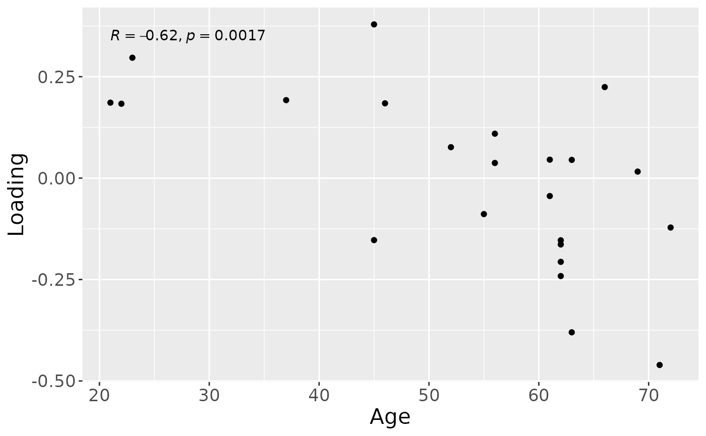
b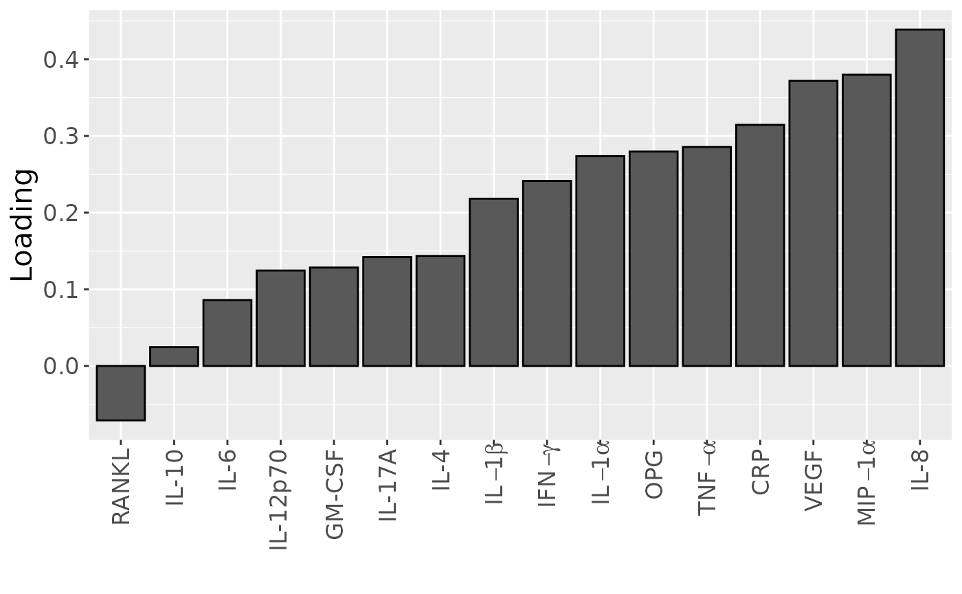
c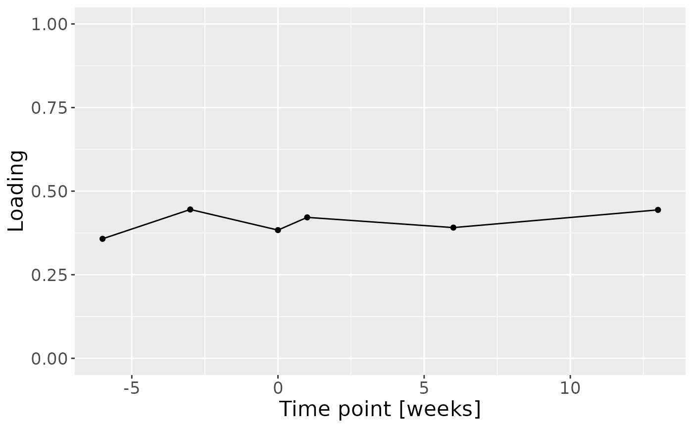
d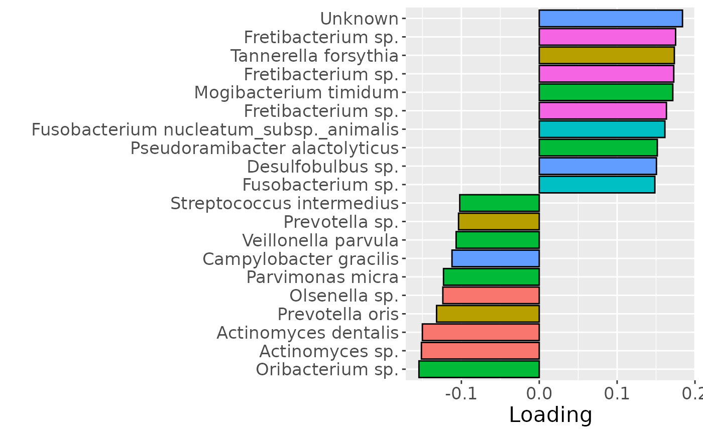
ACMTF-R
Processing
# Microbiome
processedMicrobiome_acmtf = CMTFtoolbox::Georgiou2025$Tooth_microbiome

# Remove samples due to low library size
mask = rowSums(processedMicrobiome_acmtf$data) > 6500
processedMicrobiome_acmtf$data = processedMicrobiome_acmtf$data[mask,]
processedMicrobiome_acmtf$mode1 = processedMicrobiome_acmtf$mode1[mask,]

# Remove duplicate samples
mask = !(processedMicrobiome_acmtf$mode1$SampleID %in% c("A11-8 36", "A11-10 17", "A11-15 17"))
processedMicrobiome_acmtf$data = processedMicrobiome_acmtf$data[mask,]
processedMicrobiome_acmtf$mode1 = processedMicrobiome_acmtf$mode1[mask,]

# Also remove subject A11-8 due to being an outlier
processedMicrobiome_acmtf$data = processedMicrobiome_acmtf$data[-23,,]
processedMicrobiome_acmtf$mode1 = processedMicrobiome_acmtf$mode1[-23,]

# CLR transformation
df = processedMicrobiome_acmtf$data + 1
geomeans = pracma::geomean(as.matrix(df), dim=2)
df_clr = log(sweep(df, 1, geomeans, FUN="/"))

# Feature filtering
sparsityThreshold = 0.5
maskA = processedMicrobiome_acmtf$mode1$PainS_NopainA == "A"
maskS = processedMicrobiome_acmtf$mode1$PainS_NopainA == "S"

dfA = processedMicrobiome_acmtf$data[maskA,]
dfS = processedMicrobiome_acmtf$data[maskS,]

sparsityA = colSums(dfA == 0) / nrow(dfA)
sparsityS = colSums(dfS == 0) / nrow(dfS)

mask = (sparsityA <= sparsityThreshold) | (sparsityS <= sparsityThreshold)

processedMicrobiome_acmtf$data = df_clr[,mask]
processedMicrobiome_acmtf$mode2 = processedMicrobiome_acmtf$mode2[mask,]

# Center and scale
processedMicrobiome_acmtf$data = sweep(processedMicrobiome_acmtf$data, 2, colMeans(processedMicrobiome_acmtf$data), FUN="-")
processedMicrobiome_acmtf$data = sweep(processedMicrobiome_acmtf$data, 2, apply(processedMicrobiome_acmtf$data, 2, sd), FUN="/")

# Cytokines
processedCytokines_acmtf = CMTFtoolbox::Georgiou2025$Inflammatory_mediators

# Select only case subjects
mask = processedCytokines_acmtf$mode1$case_control == "case"
processedCytokines_acmtf$data = processedCytokines_acmtf$data[mask,,]
processedCytokines_acmtf$mode1 = processedCytokines_acmtf$mode1[mask,]

# Select only samples with corresponding microbiome data
mask = processedCytokines_acmtf$mode1$SubjectID %in% processedMicrobiome_acmtf$mode1$SubjectID
processedCytokines_acmtf$data = processedCytokines_acmtf$data[mask,,]
processedCytokines_acmtf$mode1 = processedCytokines_acmtf$mode1[mask,]

processedCytokines_acmtf$data = log(processedCytokines_acmtf$data + 0.005)
processedCytokines_acmtf$data = multiwayCenter(processedCytokines_acmtf$data, 1)
processedCytokines_acmtf$data = multiwayScale(processedCytokines_acmtf$data, 2)
Y = as.numeric(as.factor(processedCytokines_case$mode1$PainS_NopainA))
Ycnt = Y - mean(Y)
Ynorm = Ycnt / norm(Ycnt, "2")
Ynorm = as.matrix(Ynorm)
Model selection
# Please see the separate R scripts at https://doi.org/10.5281/zenodo.16993009 for the model selection.
acmtfr_model90 = readRDS("./AP/AP_ACMTFR_model_90.RDS")
acmtfr_model90$varExp
#> [1]  5.937628 20.520930
Description
ACMTF-R was applied to supervise the joint decomposition using pain perception as the dependent variable (). The model selection procedure revealed that one component was appropriate for all tested values, based on a low RMSECV (Supplementary Figure~). Subsequently, the one-component ACMTF-R model using was selected for further interpretation due to balancing explaining the independent data and predicting (Supplementary Table~).
The Lambda-matrix of the model revealed that the component was predominantly distinct to the microbiome block (), with a minor contribution from the inflammatory mediator block (). MLR analysis revealed that the ACMTF-R component captured variation strongly associated with pain perception (), and weakly associated with gender (). This component was further interpreted.
testMetadata(acmtfr_model90, 1, processedCytokines_acmtf)
#>             Term   Estimate                                          CI
#> 1         Gender  98.159830      0.0135392537532894 – 0.182780405453039
#> 2            Age  -2.467714 -0.00533387362284289 – 0.000398444801317704
#> 3 PainS_NopainAS 348.687033       0.263240754458483 – 0.434133311238564
#>        P_value     P_adjust
#> 1 2.529062e-02 3.793593e-02
#> 2 8.742526e-02 8.742526e-02
#> 3 6.254957e-08 1.876487e-07
lambda = abs(acmtfr_model90$Fac[[5]])
colnames(lambda) = paste0("C", 1)

lambda %>%
  as_tibble() %>%
  mutate(block=c("cytokines", "microbiome")) %>%
  mutate(block=factor(block, levels=c("cytokines", "microbiome"))) %>%
  pivot_longer(-block) %>%
  ggplot(aes(x=as.factor(name),y=value,fill=as.factor(block))) +
  geom_bar(stat="identity",position=position_dodge(),col="black") +
  xlab("ACMTF-R component number") +
  ylab(expression(lambda)) +
  scale_x_discrete(labels=1:3) +
  scale_fill_manual(name="Dataset",values = hue_pal()(2),labels=c("Inflammatory mediators", "Tooth microbiome")) +
  theme(legend.position="top", text=element_text(size=16))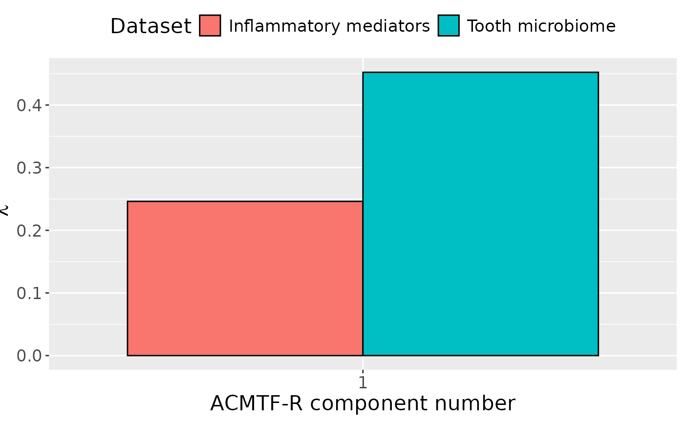
# Cytokines
topIndices = processedCytokines_case$mode2 %>% mutate(index=1:nrow(.), Comp = acmtfr_model90$Fac[[2]][,1]) %>% arrange(desc(Comp)) %>% head() %>% select(index) %>% pull()
bottomIndices = processedCytokines_case$mode2 %>% mutate(index=1:nrow(.), Comp = acmtfr_model90$Fac[[2]][,1]) %>% arrange(desc(Comp)) %>% tail() %>% select(index) %>% pull()

Xhat = parafac4microbiome::reinflateTensor(acmtfr_model90$Fac[[1]][,1], acmtfr_model90$Fac[[2]][,1], acmtfr_model90$Fac[[3]][,1])

print("Positive loadings:")
#> [1] "Positive loadings:"
print(cor(Xhat[,topIndices[1],2], as.numeric(as.factor(processedCytokines_case$mode1$PainS_NopainA)), use="pairwise.complete.obs")) # flip
#> [1] -0.8591682
print("Negative loadings:")
#> [1] "Negative loadings:"
print(cor(Xhat[,bottomIndices[6],2], as.numeric(as.factor(processedCytokines_case$mode1$PainS_NopainA)), use="pairwise.complete.obs"))
#> [1] 0.8591682

# Microbiome
topIndices = processedMicrobiome$mode2 %>% mutate(index=1:nrow(.), Comp = acmtfr_model90$Fac[[4]][,1]) %>% arrange(desc(Comp)) %>% head() %>% select(index) %>% pull()
bottomIndices = processedMicrobiome$mode2 %>% mutate(index=1:nrow(.), Comp = acmtfr_model90$Fac[[4]][,1]) %>% arrange(desc(Comp)) %>% tail() %>% select(index) %>% pull()

Xhat = CMTFtoolbox::reinflateMatrix(acmtfr_model90$Fac[[1]][,1], acmtfr_model90$Fac[[4]][,1])

print("Positive loadings:")
#> [1] "Positive loadings:"
print(cor(Xhat[,topIndices[1]], as.numeric(as.factor(processedCytokines_case$mode1$PainS_NopainA)), use="pairwise.complete.obs")) # no flip
#> [1] 0.8591682
print("Negative loadings:")
#> [1] "Negative loadings:"
print(cor(Xhat[,bottomIndices[1]], as.numeric(as.factor(processedCytokines_case$mode1$PainS_NopainA)), use="pairwise.complete.obs"))
#> [1] -0.8591682
# Subject mode
a = processedCytokines_case$mode1 %>%
  mutate(Comp1 = acmtfr_model90$Fac[[1]][,1]) %>%
  ggplot(aes(x=as.factor(PainS_NopainA),y=Comp1)) +
  geom_boxplot() +
  geom_jitter(height=0, width=0.05) +
  stat_compare_means(comparisons=list(c("A", "S")),label="p.signif") +
  xlab("") +
  ylab("Loading") +
  scale_x_discrete(labels=c("Asymptomatic", "Symptomatic")) +
  theme(text=element_text(size=16))

## Cytokines
temp = processedCytokines_case$mode2 %>%
  as_tibble() %>%
  mutate(Component_1 = -1*acmtfr_model90$Fac[[2]][,1]) %>%
  arrange(Component_1) %>%
  mutate(index=1:nrow(.))

b=temp %>%
  ggplot(aes(x=as.factor(index),y=Component_1)) +
  geom_bar(stat="identity",col="black") +
  scale_x_discrete(label=temp$name) +
  xlab("") +
  ylab("Loading") +
  scale_x_discrete(labels=c("OPG", "IL-4", "IL-6", expression(IL-1*beta), "IL-10", "IL-12p70", "VEGF", expression(IFN-gamma), "IL-17A", "GM-CSF", expression(IL-1*alpha), "IL-8", "CRP", expression(TNF-alpha), expression(MIP-1*alpha), "RANKL")) +
  theme(text=element_text(size=16),axis.text.x = element_text(angle = 90, vjust = 0.5, hjust=1))
#> Scale for x is already present.
#> Adding another scale for x, which will replace the existing scale.

# Microbiome
temp = processedMicrobiome$mode2 %>%
  mutate(comp=acmtfr_model90$Fac[[4]][,1]) %>%
  mutate(Phylum = as.factor(str_split_fixed(Phylum, "__", 2)[,2]),
         Genus = str_split_fixed(Genus,"g__",2)[,2],
         Species = str_split_fixed(Species,"s__",2)[,2]) %>%
  arrange(comp) %>%
  mutate(index=1:nrow(.)) %>%
  filter(index %in% c(1:10, 143:152))

temp[temp$Species == "","Species"] = "sp."
temp[grepl("taxon", temp$Species), "Species"] = "sp."
temp$name = paste0(temp$Genus, " ", temp$Species)
temp[temp$name == " sp.","name"] = "Unknown"

c = temp %>%
  ggplot(aes(x=comp,y=as.factor(index),fill=Phylum)) +
  geom_bar(stat="identity", col="black") +
  scale_y_discrete(label=temp$name) +
  xlab("Loading") +
  ylab("") +
  scale_fill_manual(name="Phylum", labels=c("Actinobacteria", "Firmicutes", "Fusobacteria"), values=hue_pal()(6)[c(1,3,4)]) +
  theme(legend.position="none", text=element_text(size=16))

d = acmtfr_model90$Fac[[3]][,1] %>%
  as_tibble() %>%
  mutate(value=-1*value) %>%
  mutate(timepoint=c(-6,-3,0,1,6,13)) %>%
  ggplot(aes(x=timepoint,y=value)) +
  geom_line() +
  geom_point() +
  xlab("Time point [weeks]") +
  ylab("Loading") +
  ylim(0,1) +
  theme(text=element_text(size=16))

a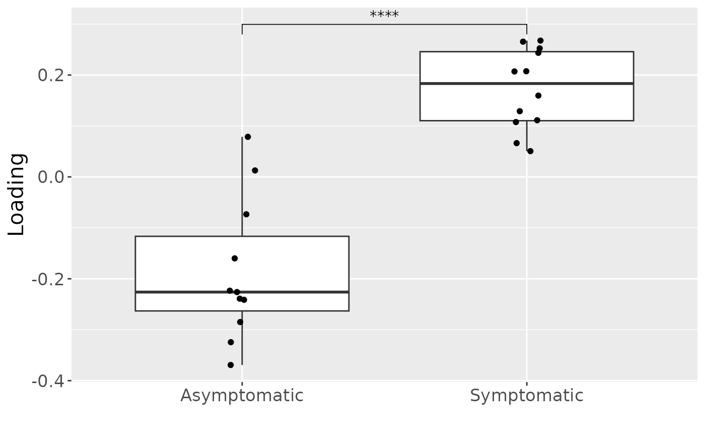
b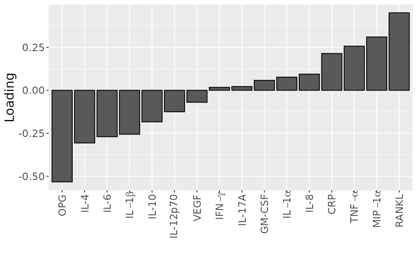
c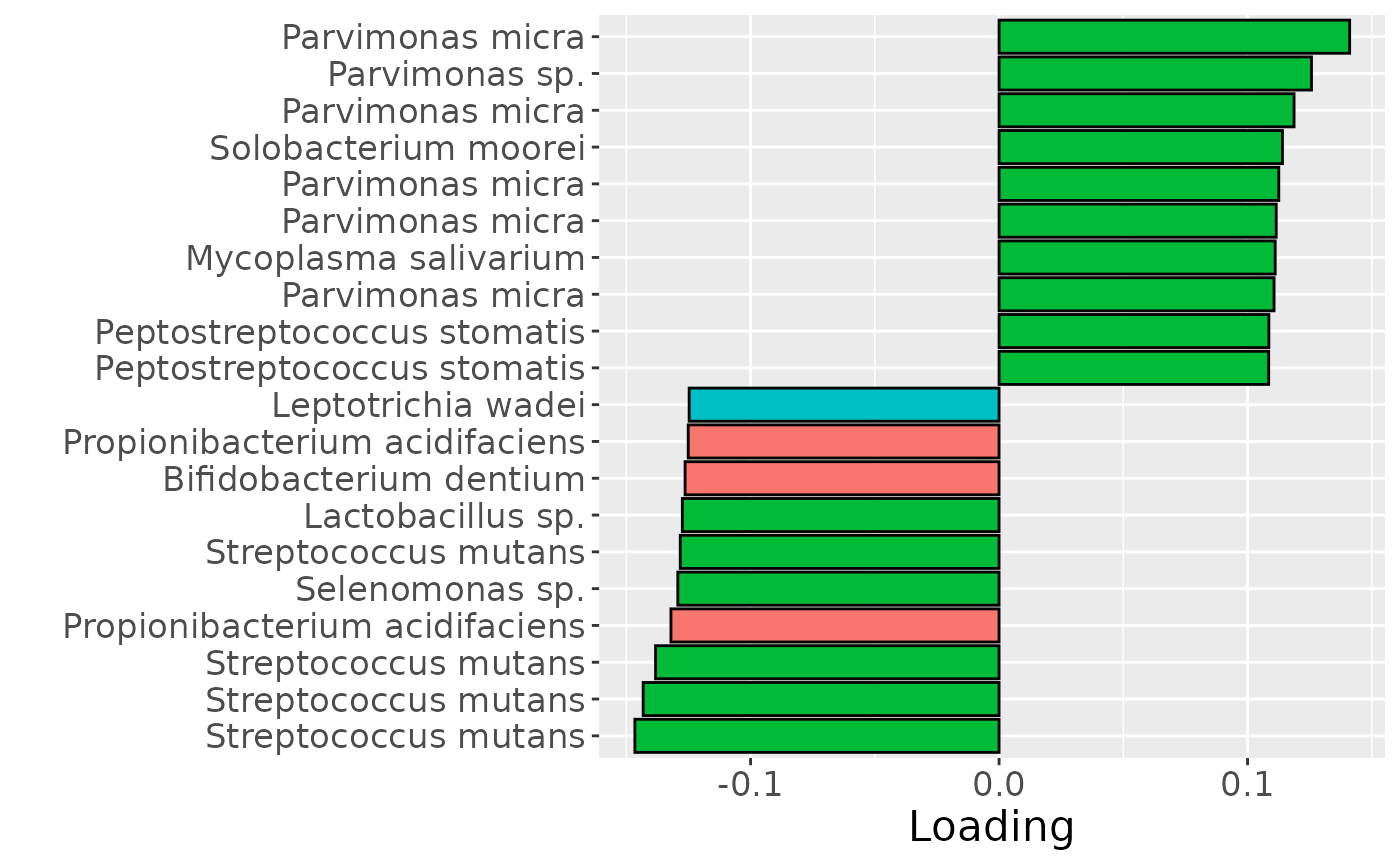
d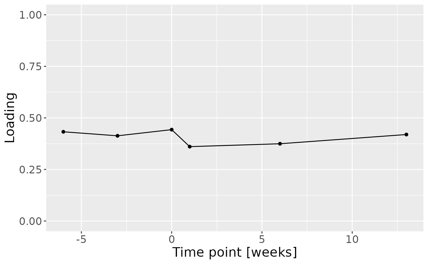
Positively loaded inflammatory mediators included RANKL, MIP-1alpha, TNF-alpha, CRP, IL-8, IL-1alpha, GM-CSF, IL-17A, and IFN-gamma, which had higher levels in symptomatic AP and lower levels in asymptomatic AP. Conversely, negatively loaded inflammatory mediators included OPG, IL-4, IL-6, IL-1beta, IL-10, IL-12p70, and VEGF, which had higher levels in asymptomatic AP and lower levels in symptomatic AP. The time mode loadings indicate that inter-subject differences were slightly larger before the tooth extraction than after the extraction.
Positively loaded microbiota included Parvimonas micra, Parvimonas sp., Solobacterium moorei, Mycoplasma salivarium, and Peptostreptococcus stomatis, which were enriched in symptomatic AP and depleted in asymptomatic AP. Conversely, negatively loaded microbiota included Streptococcus mutans, Propionibacterium acidifaciens, Selenomonas sp., Lactobacillus sp., Bifidobacterium dentium, and Leptotrichia wadei, which were enriched in asymptomatic AP and depleted in symptomatic AP. These associations largely align with the previously presented PLS and NPLS results, but are confounded by age to some degree.