GOHTRANS: gender-affirming hormone therapy
2025-08-31
Source:vignettes/articles/GOHTRANS.Rmd
GOHTRANS.RmdPreamble
library(dplyr)
#>
#> Attaching package: 'dplyr'
#> The following objects are masked from 'package:stats':
#>
#>     filter, lag
#> The following objects are masked from 'package:base':
#>
#>     intersect, setdiff, setequal, union
library(tidyr)
library(parafac4microbiome)
library(NPLStoolbox)
library(CMTFtoolbox)
#>
#> Attaching package: 'CMTFtoolbox'
#> The following object is masked from 'package:NPLStoolbox':
#>
#>     npred
#> The following objects are masked from 'package:parafac4microbiome':
#>
#>     fac_to_vect, reinflateFac, reinflateTensor, vect_to_fac
library(ggplot2)
library(ggpubr)
library(readr)
library(stringr)
library(scales)
#>
#> Attaching package: 'scales'
#> The following object is masked from 'package:readr':
#>
#>     col_factor
ph_BOMP = read_delim("./GOHTRANS/GOH-TRANS_export_20240205.csv",
                     delim = ";", escape_double = FALSE, trim_ws = TRUE) %>% as_tibble()
#> Rows: 42 Columns: 347
#> ── Column specification ────────────────────────────────────────────────────────
#> Delimiter: ";"
#> chr (104): Participant Status, Site Abbreviation, Participant Creation Date,...
#> dbl (243): Participant Id, pat_genderID, Age, Informed_consent#Yes, Informed...
#>
#> ℹ Use `spec()` to retrieve the full column specification for this data.
#> ℹ Specify the column types or set `show_col_types = FALSE` to quiet this message.

df1 = ph_BOMP %>% select(`Participant Id`, starts_with("5.")) %>% mutate(subject = 1:42, numTeeth = `5.1|Number of teeth`, DMFT = `5.2|DMFT`, numBleedingSites = `5.3|Bleeding sites`, boppercent = `5.4|BOP%`, DPSI = `5.5|DPSI`, pH = `5.8|pH`) %>% select(subject, numTeeth, DMFT, numBleedingSites, boppercent, DPSI, pH)
df2 = ph_BOMP %>% select(`Participant Id`, starts_with("12.")) %>% mutate(subject = 1:42, numTeeth = `12.1|Number of teeth`, DMFT = `12.2|DMFT`, numBleedingSites = `12.3|Bleeding sites`, boppercent = `12.4|BOP%`, DPSI = `12.5|DPSI`, pH = `12.8|pH`) %>% select(subject, numTeeth, DMFT, numBleedingSites, boppercent, DPSI, pH)
df3 = ph_BOMP %>% select(`Participant Id`, starts_with("19.")) %>% mutate(subject = 1:42, numTeeth = `19.1|Number of teeth`, DMFT = `19.2|DMFT`, numBleedingSites = `19.3|Bleeding sites`, boppercent = `19.4|BOP%`, DPSI = `19.5|DPSI`, pH = `19.8|pH`) %>% select(subject, numTeeth, DMFT, numBleedingSites, boppercent, DPSI, pH)
df4 = ph_BOMP %>% select(`Participant Id`, starts_with("26.")) %>% mutate(subject = 1:42, numTeeth = `26.1|Number of teeth`, DMFT = `26.2|DMFT`, numBleedingSites = `26.3|Bleeding sites`, boppercent = `26.4|BOP%`, DPSI = `26.5|DPSI`, pH = `26.8|pH`) %>% select(subject, numTeeth, DMFT, numBleedingSites, boppercent, DPSI, pH)

otherMeta = rbind(df1, df2, df3, df4) %>% as_tibble() %>% mutate(newTimepoint = rep(c(0,3,6,12), each=42))
otherMeta = otherMeta %>% select(subject, newTimepoint, boppercent)
otherMeta[otherMeta$boppercent < 0 & !is.na(otherMeta$boppercent), "boppercent"] = NA

saliva_sampleMeta = read.csv("./GOHTRANS/sampleInfo_fixed.csv", sep=" ") %>% as_tibble() %>% select(subject, GenderID, Age, newTimepoint)

# CODS XI
df = read.csv("./GOHTRANS/CODS_XI.csv")
df = df[1:40,1:10] %>% as_tibble() %>% filter(Participant_code %in% saliva_sampleMeta$subject)

CODS = df %>% select(Participant_code, CODS_BASELINE, CODS_3_MONTHS, CODS_6_MONTHS, CODS_12_MONTHS) %>% pivot_longer(-Participant_code) %>% mutate(timepoint = NA)
CODS[CODS$name == "CODS_BASELINE", "timepoint"] = 0
CODS[CODS$name == "CODS_3_MONTHS", "timepoint"] = 3
CODS[CODS$name == "CODS_6_MONTHS", "timepoint"] = 6
CODS[CODS$name == "CODS_12_MONTHS", "timepoint"] = 12
CODS[CODS$value == -99, "value"] = NA
CODS = CODS %>% mutate(subject = Participant_code, newTimepoint = timepoint, CODS = value) %>% select(-Participant_code, -name, -value, -timepoint)

XI = df %>% select(Participant_code, XI_BASELINE, XI_3_MONTHS, XI_6_MONTHS, XI_12_MONTHS) %>% pivot_longer(-Participant_code) %>% mutate(timepoint = NA)
XI[XI$name == "XI_BASELINE", "timepoint"] = 0
XI[XI$name == "XI_3_MONTHS", "timepoint"] = 3
XI[XI$name == "XI_6_MONTHS", "timepoint"] = 6
XI[XI$name == "XI_12_MONTHS", "timepoint"] = 12
XI[XI$value == -99, "value"] = NA
XI = XI %>% mutate(subject = Participant_code, newTimepoint = timepoint, XI = value) %>% select(-Participant_code, -name, -value, -timepoint)

df = otherMeta %>% left_join(CODS) %>% left_join(XI) %>% select(subject, newTimepoint, boppercent, CODS, XI) %>% filter(newTimepoint != "NA")
#> Joining with `by = join_by(subject, newTimepoint)`
#> Joining with `by = join_by(subject, newTimepoint)`

meta = df %>% left_join(otherMeta) %>% left_join(saliva_sampleMeta) %>% filter(newTimepoint==12) %>% unique() %>% select(-newTimepoint)
#> Joining with `by = join_by(subject, newTimepoint, boppercent)`
#> Joining with `by = join_by(subject, newTimepoint)`
meta[meta < 0] <- NA

newBOP = residuals(lm(boppercent ~ GenderID + Age + CODS + XI, data=meta, na.action=na.exclude))
newCODS= residuals(lm(CODS ~ boppercent + GenderID + Age + XI, data=meta, na.action=na.exclude))
newXI = residuals(lm(XI ~ boppercent + GenderID + Age + CODS, data=meta, na.action=na.exclude))

meta = meta %>% mutate(boppercent = newBOP, CODS = newCODS, XI = newXI)
prepMetadata = function(model, metadata){
  longA = parafac4microbiome::transformPARAFACloadings(model$Fac, 2, moreOutput = TRUE)$F
  df = longA %>% as_tibble() %>% mutate(subject=as.integer(rep(metadata$mode1$subject, each=nrow(metadata$mode3))), newTimepoint = rep(metadata$mode3$newTimepoint, nrow(metadata$mode1))) %>% left_join(Cornejo2025$Blood_hormones) %>% left_join(Cornejo2025$Clinical_measurements)

  newTesto = residuals(lm(Free_testosterone_Vermeulen_pmol_L ~ Estradiol_pmol_ml + LH_U_L + SHBG_nmol_L + boppercent + pH + GenderID + Age, data=df, na.action=na.exclude))
  newEstra = residuals(lm(Estradiol_pmol_ml ~ Free_testosterone_Vermeulen_pmol_L + LH_U_L + SHBG_nmol_L + boppercent + pH + GenderID + Age, data=df, na.action=na.exclude))
  newLH = residuals(lm(LH_U_L ~ Free_testosterone_Vermeulen_pmol_L + Estradiol_pmol_ml + SHBG_nmol_L + boppercent + pH + GenderID + Age, data=df, na.action=na.exclude))
  newSHBG = residuals(lm(SHBG_nmol_L ~ Free_testosterone_Vermeulen_pmol_L + Estradiol_pmol_ml + LH_U_L + boppercent + pH + GenderID + Age, data=df, na.action=na.exclude))
  newBOP = residuals(lm(boppercent ~ Free_testosterone_Vermeulen_pmol_L + Estradiol_pmol_ml + LH_U_L + SHBG_nmol_L + pH + GenderID + Age, data=df, na.action=na.exclude))
  newPH = residuals(lm(pH ~ Free_testosterone_Vermeulen_pmol_L + Estradiol_pmol_ml + LH_U_L + SHBG_nmol_L + boppercent + GenderID + Age, data=df, na.action=na.exclude))

  df$Free_testosterone_Vermeulen_pmol_L = newTesto
  df$Estradiol_pmol_ml = newEstra
  df$LH_U_L = newLH
  df$SHBG_nmol_L = newSHBG
  df$boppercent = newBOP
  df$pH = newPH
  df$GenderID = as.numeric(as.factor(df$GenderID))

  return(df)
}

clinical_metadata = NPLStoolbox::Cornejo2025$Clinical_measurements$mode1 %>% mutate(BOP = NPLStoolbox::Cornejo2025$Clinical_measurements$data[,1,2], CODS = NPLStoolbox::Cornejo2025$Clinical_measurements$data[,2,2], XI = NPLStoolbox::Cornejo2025$Clinical_measurements$data[,3,2]) %>% left_join(NPLStoolbox::Cornejo2025$Subject_metadata %>% mutate(subject = as.character(subject)))
#> Joining with `by = join_by(subject, GenderID)`

testMetadata = function(model, comp, metadata){
  transformedSubjectLoadings = model$Fac[[1]][,comp]
  transformedSubjectLoadings = transformedSubjectLoadings / norm(transformedSubjectLoadings, "2")

  metadata = metadata$mode1 %>% left_join(clinical_metadata) %>% mutate(GenderID = as.numeric(as.factor(GenderID))-1)

  result = lm(transformedSubjectLoadings ~ GenderID + Age + BOP + CODS + XI, data=metadata)

  # Extract coefficients and confidence intervals
  coef_estimates <- summary(result)$coefficients
  conf_intervals <- confint(result)

  # Remove intercept
  coef_estimates <- coef_estimates[rownames(coef_estimates) != "(Intercept)", ]
  conf_intervals <- conf_intervals[rownames(conf_intervals) != "(Intercept)", ]

  # Combine into a clean data frame
  summary_table <- data.frame(
    Term     = rownames(coef_estimates),
    Estimate = coef_estimates[, "Estimate"] * 1e3,
    CI       = paste0(
                 conf_intervals[, 1], " – ",
                 conf_intervals[, 2]
               ),
    P_value  = coef_estimates[, "Pr(>|t|)"],
    P_adjust = p.adjust(coef_estimates[, "Pr(>|t|)"], "BH"),
    row.names = NULL
  )

  return(summary_table)
}
processedTongue = processDataCube(NPLStoolbox::Cornejo2025$Tongue_microbiome, sparsityThreshold = 0.5, considerGroups=TRUE, groupVariable="GenderID", CLR=TRUE, centerMode=1, scaleMode=2)
processedSaliva = processDataCube(NPLStoolbox::Cornejo2025$Salivary_microbiome, sparsityThreshold = 0.5, considerGroups=TRUE, groupVariable="GenderID", CLR=TRUE, centerMode=1, scaleMode=2)

processedCytokines = NPLStoolbox::Cornejo2025$Salivary_cytokines
processedCytokines$data = log(processedCytokines$data + 0.1300)
# Remove subject 1, 18, 19, and 27 due to being an outlier
processedCytokines$data = processedCytokines$data[-c(1,9,10,19),,]
processedCytokines$mode1 = processedCytokines$mode1[-c(1,9,10,19),]
processedCytokines$data = multiwayCenter(processedCytokines$data, 1)
processedCytokines$data = multiwayScale(processedCytokines$data, 2)

processedBiochemistry = NPLStoolbox::Cornejo2025$Salivary_biochemistry
processedBiochemistry$data = log(processedBiochemistry$data)
processedBiochemistry$data = multiwayCenter(processedBiochemistry$data, 1)
processedBiochemistry$data = multiwayScale(processedBiochemistry$data, 2)

processedHormones = NPLStoolbox::Cornejo2025$Circulatory_hormones
processedHormones$data = log(processedHormones$data)
processedHormones$data = multiwayCenter(processedHormones$data, 1)
processedHormones$data = multiwayScale(processedHormones$data, 2)
deltaT = NPLStoolbox::Cornejo2025$Circulatory_hormones$data[,1,2] - NPLStoolbox::Cornejo2025$Circulatory_hormones$data[,1,1]
outcome = processedHormones$mode1 %>% mutate(deltaT = deltaT) %>% filter(deltaT != "NA")
processedTongue = processDataCube(NPLStoolbox::Cornejo2025$Tongue_microbiome, sparsityThreshold = 0.5, considerGroups=TRUE, groupVariable="GenderID", CLR=TRUE, centerMode=FALSE, scaleMode=FALSE)
mask = processedTongue$mode1$subject %in% outcome$subject
processedTongue$mode1 = processedTongue$mode1[mask,]
processedTongue$data = processedTongue$data[mask,,]
processedTongue$data = multiwayCenter(processedTongue$data, 1)
processedTongue$data = multiwayScale(processedTongue$data, 2)

processedSaliva = processDataCube(NPLStoolbox::Cornejo2025$Salivary_microbiome, sparsityThreshold = 0.5, considerGroups=TRUE, groupVariable="GenderID", CLR=TRUE, centerMode=1, scaleMode=2)
mask = processedSaliva$mode1$subject %in% outcome$subject
processedSaliva$mode1 = processedSaliva$mode1[mask,]
processedSaliva$data = processedSaliva$data[mask,,]
processedSaliva$data = multiwayCenter(processedSaliva$data, 1)
processedSaliva$data = multiwayScale(processedSaliva$data, 2)

processedCytokines = NPLStoolbox::Cornejo2025$Salivary_cytokines
processedCytokines$data = log(processedCytokines$data + 0.1300)
# Remove subject 1, 18, 19, and 27 due to being an outlier
processedCytokines$data = processedCytokines$data[-c(1,9,10,19),,]
processedCytokines$mode1 = processedCytokines$mode1[-c(1,9,10,19),]
mask = processedCytokines$mode1$subject %in% outcome$subject
processedCytokines$mode1 = processedCytokines$mode1[mask,]
processedCytokines$data = processedCytokines$data[mask,,]
processedCytokines$data = multiwayCenter(processedCytokines$data, 1)
processedCytokines$data = multiwayScale(processedCytokines$data, 2)

processedBiochemistry = NPLStoolbox::Cornejo2025$Salivary_biochemistry
processedBiochemistry$data = log(processedBiochemistry$data)
mask = processedBiochemistry$mode1$subject %in% outcome$subject
processedBiochemistry$mode1 = processedBiochemistry$mode1[mask,]
processedBiochemistry$data = processedBiochemistry$data[mask,,]
processedBiochemistry$data = multiwayCenter(processedBiochemistry$data, 1)
processedBiochemistry$data = multiwayScale(processedBiochemistry$data, 2)
Y = processedTongue$mode1 %>% left_join(outcome) %>% select(deltaT) %>% pull()
#> Joining with `by = join_by(subject, GenderID)`
Ycnt = Y - mean(Y)
Ynorm_tongue = Ycnt / norm(Ycnt, "2")

Y = processedSaliva$mode1 %>% left_join(outcome) %>% select(deltaT) %>% pull()
#> Joining with `by = join_by(subject, GenderID)`
Ycnt = Y - mean(Y)
Ynorm_saliva = Ycnt / norm(Ycnt, "2")

Y = processedCytokines$mode1 %>% left_join(outcome) %>% select(deltaT) %>% pull()
#> Joining with `by = join_by(subject, GenderID)`
Ycnt = Y - mean(Y)
Ynorm_cytokine = Ycnt / norm(Ycnt, "2")

Y = processedBiochemistry$mode1 %>% left_join(outcome) %>% select(deltaT) %>% pull()
#> Joining with `by = join_by(subject, GenderID)`
Ycnt = Y - mean(Y)
Ynorm_biochem = Ycnt / norm(Ycnt, "2")
ACMTF
Processing
deltaT = NPLStoolbox::Cornejo2025$Circulatory_hormones$data[,1,2] - NPLStoolbox::Cornejo2025$Circulatory_hormones$data[,1,1]
outcome = NPLStoolbox::Cornejo2025$Circulatory_hormones$mode1 %>% mutate(deltaT = deltaT) %>% filter(deltaT != "NA")

homogenizedSamples1 = intersect(NPLStoolbox::Cornejo2025$Tongue_microbiome$mode1$subject, outcome$subject)
homogenizedSamples2 = intersect(NPLStoolbox::Cornejo2025$Salivary_microbiome$mode1$subject, outcome$subject)
homogenizedSamples3 = intersect(NPLStoolbox::Cornejo2025$Salivary_cytokines$mode1$subject, outcome$subject)
homogenizedSamples4 = intersect(NPLStoolbox::Cornejo2025$Salivary_biochemistry$mode1$subject, outcome$subject)

homogenizedSamples = intersect(intersect(homogenizedSamples1, homogenizedSamples2), intersect(homogenizedSamples3,homogenizedSamples4))

outcome = outcome %>% filter(subject %in% homogenizedSamples)

# Tongue
newTongue = NPLStoolbox::Cornejo2025$Tongue

mask = newTongue$mode1$subject %in% homogenizedSamples
newTongue$data = newTongue$data[mask,,]
newTongue$mode1 = newTongue$mode1[mask,]

processedTongue_acmtf = processDataCube(newTongue, sparsityThreshold = 0.5, considerGroups=TRUE, groupVariable="GenderID", CLR=TRUE, centerMode=1, scaleMode=2)

# Saliva
newSaliva = NPLStoolbox::Cornejo2025$Salivary_microbiome

mask = newSaliva$mode1$subject %in% homogenizedSamples
newSaliva$data = newSaliva$data[mask,,]
newSaliva$mode1 = newSaliva$mode1[mask,]

processedSaliva_acmtf = processDataCube(newSaliva, sparsityThreshold = 0.5, considerGroups=TRUE, groupVariable="GenderID", CLR=TRUE, centerMode=1, scaleMode=2)

# Cytokines
newCytokines = NPLStoolbox::Cornejo2025$Salivary_cytokines

mask = newCytokines$mode1$subject %in% homogenizedSamples
newCytokines$data = log(newCytokines$data[mask,,] + 0.1300)
newCytokines$mode1 = newCytokines$mode1[mask,]

processedCytokines_acmtf = processDataCube(newCytokines, CLR=FALSE, centerMode=1, scaleMode=2)

# Biochemistry
newBio = NPLStoolbox::Cornejo2025$Salivary_biochemistry

mask = newBio$mode1$subject %in% homogenizedSamples
newBio$data = log(newBio$data[mask,,])
newBio$mode1 = newBio$mode1[mask,]

processedBiochemistry_acmtf = processDataCube(newBio, CLR=FALSE, centerMode=1, scaleMode=2)
# Please see the separate R scripts at https://doi.org/10.5281/zenodo.16993009 for the model selection.
acmtf_model = readRDS("./GOHTRANS/GOHTRANS_ACMTFR_model_1_deltaT.RDS")
acmtf_model$varExp
#> [1] 12.26085 10.83131 50.10408 19.93142
Description
ACMTF was applied to the capture to dominant source of variation across all data blocks. The model selection procedure revealed that FMS CV < 0.9 when three components were selected. Therefore, a two-component ACMTF model was selected, explaining 12.3%, 10.8%, 50.1%, and 19.9% of the variation in the tongue microbiome, salivary microbiome, salivary cytokine, and salivary biochemistry data blocks, respectively. The Lambda-matrix of the model revealed that the first component was distinct to the salivary cytokine block, while the second component was predominantly distinct to the salivary biochemistry block. MLR analysis revealed that the first component was uninterpretable, while the second component was weakly associated with gender identity.
testMetadata(acmtf_model, 1, processedTongue_acmtf)
#> Joining with `by = join_by(subject, GenderID)`
#>       Term      Estimate                                        CI    P_value
#> 1 GenderID -101.21791354   -0.290530383376818 – 0.0880945562890892 0.27497424
#> 2      Age   -0.02948517  -0.0209679087018061 – 0.0209089383631103 0.99766407
#> 3      BOP    3.79594066 -0.00978973512676411 – 0.0173816164549634 0.56328018
#> 4     CODS  195.59611322   -0.0171112553246807 – 0.408303481755385 0.06914254
#> 5       XI    4.28194458  -0.0180263793638558 – 0.0265902685172408 0.69055280
#>    P_adjust
#> 1 0.6874356
#> 2 0.9976641
#> 3 0.8631910
#> 4 0.3457127
#> 5 0.8631910
testMetadata(acmtf_model, 2, processedTongue_acmtf)
#> Joining with `by = join_by(subject, GenderID)`
#>       Term    Estimate                                        CI    P_value
#> 1 GenderID  226.449388    0.0421578238420423 – 0.410740952272122 0.01897398
#> 2      Age    5.034403    -0.015348696173811 – 0.025417501936632 0.60901796
#> 3      BOP    5.583413 -0.00764194599027333 – 0.0188087727038087 0.38551700
#> 4     CODS -175.966485   -0.383032473273648 – 0.0310995033774118 0.09079355
#> 5       XI   -8.462002  -0.0301786687708441 – 0.0132546657331868 0.42240150
#>     P_adjust
#> 1 0.09486989
#> 2 0.60901796
#> 3 0.52800187
#> 4 0.22698387
#> 5 0.52800187
lambda = abs(acmtf_model$Fac[[10]])
colnames(lambda) = paste0("C", 1:2)

lambda %>%
  as_tibble() %>%
  mutate(block=c("tongue", "saliva", "cytokines", "biochemistry")) %>%
  mutate(block=factor(block, levels=c("tongue", "saliva", "cytokines", "biochemistry"))) %>%
  pivot_longer(-block) %>%
  ggplot(aes(x=as.factor(name),y=value,fill=as.factor(block))) +
  geom_bar(stat="identity",position=position_dodge(),col="black") +
  xlab("ACMTF component number") +
  ylab(expression(lambda)) +
  scale_x_discrete(labels=1:3) +
  scale_fill_manual(name="Dataset",values = hue_pal()(4),labels=c("Tongue", "Salivary microbiome", "Salivary cytokines", "Salivary biochemistry")) +
  theme(legend.position="top")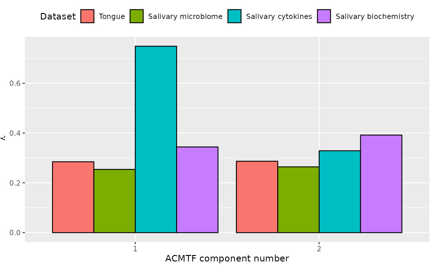
# Briefly check how the signs work

# Tongue
topIndices = processedTongue_acmtf$mode2 %>% mutate(index=1:nrow(.), Comp = acmtf_model$Fac[[2]][,2]) %>% arrange(desc(Comp)) %>% head() %>% select(index) %>% pull()
bottomIndices = processedTongue_acmtf$mode2 %>% mutate(index=1:nrow(.), Comp = acmtf_model$Fac[[2]][,2]) %>% arrange(desc(Comp)) %>% tail() %>% select(index) %>% pull()

Xhat = parafac4microbiome::reinflateTensor(acmtf_model$Fac[[1]][,2], acmtf_model$Fac[[2]][,2], acmtf_model$Fac[[3]][,2])

print("Positive loadings:") # flip
#> [1] "Positive loadings:"
print(cor(Xhat[,topIndices[1],1], as.numeric(as.factor(processedTongue_acmtf$mode1$GenderID)), use="pairwise.complete.obs"))
#> [1] -0.3927546
processedTongue_acmtf$mode1 %>% mutate(comp = Xhat[,topIndices[1],1]) %>% ggplot(aes(x=as.factor(GenderID),y=comp)) + geom_boxplot()
print("Negative loadings:")
#> [1] "Negative loadings:"
print(cor(Xhat[,bottomIndices[1],1], as.numeric(as.factor(processedTongue_acmtf$mode1$GenderID)), use="pairwise.complete.obs"))
#> [1] 0.3927546
processedTongue_acmtf$mode1 %>% mutate(comp = Xhat[,bottomIndices[1],1]) %>% ggplot(aes(x=as.factor(GenderID),y=comp)) + geom_boxplot()
# Saliva
topIndices = processedSaliva_acmtf$mode2 %>% mutate(index=1:nrow(.), Comp = acmtf_model$Fac[[4]][,2]) %>% arrange(desc(Comp)) %>% head() %>% select(index) %>% pull()
bottomIndices = processedSaliva_acmtf$mode2 %>% mutate(index=1:nrow(.), Comp = acmtf_model$Fac[[4]][,2]) %>% arrange(desc(Comp)) %>% tail() %>% select(index) %>% pull()

Xhat = parafac4microbiome::reinflateTensor(acmtf_model$Fac[[1]][,2], acmtf_model$Fac[[4]][,2], acmtf_model$Fac[[5]][,2])

print("Positive loadings:")
#> [1] "Positive loadings:"
print(cor(Xhat[,topIndices[1],1], as.numeric(as.factor(processedSaliva_acmtf$mode1$GenderID)), use="pairwise.complete.obs")) #flip
#> [1] -0.3927546
processedSaliva_acmtf$mode1 %>% mutate(comp = Xhat[,topIndices[1],1]) %>% ggplot(aes(x=as.factor(GenderID),y=comp)) + geom_boxplot()
print("Negative loadings:")
#> [1] "Negative loadings:"
print(cor(Xhat[,bottomIndices[1],1], as.numeric(as.factor(processedSaliva_acmtf$mode1$GenderID)), use="pairwise.complete.obs"))
#> [1] 0.3927546
processedSaliva_acmtf$mode1 %>% mutate(comp = Xhat[,bottomIndices[1],1]) %>% ggplot(aes(x=as.factor(GenderID),y=comp)) + geom_boxplot()
# Cytokines
topIndices = processedCytokines_acmtf$mode2 %>% mutate(index=1:nrow(.), Comp = acmtf_model$Fac[[6]][,2]) %>% arrange(desc(Comp)) %>% head() %>% select(index) %>% pull()
bottomIndices = processedCytokines_acmtf$mode2 %>% mutate(index=1:nrow(.), Comp = acmtf_model$Fac[[6]][,2]) %>% arrange(desc(Comp)) %>% tail() %>% select(index) %>% pull()

Xhat = -0.33 * parafac4microbiome::reinflateTensor(acmtf_model$Fac[[1]][,2], acmtf_model$Fac[[6]][,2], acmtf_model$Fac[[7]][,2])

print("Positive loadings:")
#> [1] "Positive loadings:"
print(cor(Xhat[,topIndices[1],1], as.numeric(as.factor(processedCytokines_acmtf$mode1$GenderID)), use="pairwise.complete.obs")) # no flip - all positive and TF associated
#> [1] 0.3927546
processedCytokines_acmtf$mode1 %>% mutate(comp = Xhat[,topIndices[1],1]) %>% ggplot(aes(x=as.factor(GenderID),y=comp)) + geom_boxplot()
print("Negative loadings:")
#> [1] "Negative loadings:"
print(cor(Xhat[,bottomIndices[6],1], as.numeric(as.factor(processedCytokines_acmtf$mode1$GenderID)), use="pairwise.complete.obs"))
#> [1] -0.3927546
processedCytokines_acmtf$mode1 %>% mutate(comp = Xhat[,bottomIndices[1],1]) %>% ggplot(aes(x=as.factor(GenderID),y=comp)) + geom_boxplot()
# Biochemistry
topIndices = 1
bottomIndices = 7

Xhat = parafac4microbiome::reinflateTensor(acmtf_model$Fac[[1]][,2], acmtf_model$Fac[[8]][,2], acmtf_model$Fac[[9]][,2])

print("Positive loadings:")
#> [1] "Positive loadings:"
print(cor(Xhat[,topIndices[1],1], as.numeric(as.factor(processedBiochemistry_acmtf$mode1$GenderID)), use="pairwise.complete.obs")) # no flip
#> [1] 0.3927546
processedBiochemistry_acmtf$mode1 %>% mutate(comp = Xhat[,topIndices[1],1]) %>% ggplot(aes(x=as.factor(GenderID),y=comp)) + geom_boxplot()
print("Negative loadings:")
#> [1] "Negative loadings:"
print(cor(Xhat[,bottomIndices[1],1], as.numeric(as.factor(processedBiochemistry_acmtf$mode1$GenderID)), use="pairwise.complete.obs"))
#> [1] -0.3927546
processedBiochemistry_acmtf$mode1 %>% mutate(comp = Xhat[,bottomIndices[1],1]) %>% ggplot(aes(x=as.factor(GenderID),y=comp)) + geom_boxplot()
# Tongue
temp = processedTongue_acmtf$mode2 %>%
  as_tibble() %>%
  mutate(Component_1 = -1*acmtf_model$Fac[[2]][,2]) %>%
  mutate(Genus = gsub("g__", "", Genus), Species = gsub("s__", "", Species)) %>%
  mutate(Species = gsub("\\(", "", Species)) %>%
  mutate(Species = gsub("\\)", "", Species))

fixedSpeciesNames = str_split_fixed(temp$Species, "/", 5) %>%
  as_tibble() %>%
  mutate(dplyr::across(.cols = everything(), .fns = ~ dplyr::if_else(stringr::str_detect(.x, "sp."), "", .x)))
#> Warning: The `x` argument of `as_tibble.matrix()` must have unique column names if
#> `.name_repair` is omitted as of tibble 2.0.0.
#> ℹ Using compatibility `.name_repair`.
#> This warning is displayed once every 8 hours.
#> Call `lifecycle::last_lifecycle_warnings()` to see where this warning was
#> generated.
fixedSpeciesNames[fixedSpeciesNames$V1 == "", "V1"] = "sp."
fixedSpeciesNames = fixedSpeciesNames %>%
  mutate(name=paste0(V1, "/", V2)) %>%
  mutate(name=gsub("/$", "", name)) %>%
  mutate(name=paste0(name, "/", V3)) %>%
  mutate(name=gsub("/$", "", name)) %>%
  mutate(name=paste0(name, "/", V4)) %>%
  mutate(name=gsub("/$", "", name)) %>%
  mutate(name=paste0(name, "/", V5)) %>%
  mutate(name=gsub("/$", "", name))

temp$Species = fixedSpeciesNames$name
temp$name = paste0(temp$Genus, " ", temp$Species)
temp[temp$name == " sp.", "name"] = "Unclassified"
temp[temp$name == " ", "name"] = "Unclassified"
temp[temp$name == " sp.", "name"] = "Unclassified"

temp = temp %>%
  arrange(Component_1) %>%
  mutate(index=1:nrow(.)) %>%
  filter(index %in% c(1:10,228:237))

a=temp %>%
  ggplot(aes(x=Component_1,y=as.factor(index),fill=as.factor(Phylum))) +
  geom_bar(stat="identity", col="black") +
  scale_y_discrete(label=temp$name) +
  xlab("Loading") +
  ylab("") +
  scale_fill_manual(name="Phylum", labels=c("Actinobacteria", "Bacteroidetes", "Firmicutes"), values=hue_pal()(5)[-c(4,5)]) +
  theme(text=element_text(size=16))

# Saliva comp 1
temp = processedSaliva_acmtf$mode2 %>%
  as_tibble() %>%
  mutate(Component_1 = -1*acmtf_model$Fac[[4]][,2]) %>%
  mutate(Genus = gsub("g__", "", Genus), Species = gsub("s__", "", Species)) %>%
  mutate(Species = gsub("\\(", "", Species)) %>%
  mutate(Species = gsub("\\)", "", Species))

fixedSpeciesNames = str_split_fixed(temp$Species, "/", 5) %>%
  as_tibble() %>%
  mutate(dplyr::across(.cols = everything(), .fns = ~ dplyr::if_else(stringr::str_detect(.x, "sp."), "", .x)))
fixedSpeciesNames[fixedSpeciesNames$V1 == "", "V1"] = "sp."
fixedSpeciesNames = fixedSpeciesNames %>%
  mutate(name=paste0(V1, "/", V2)) %>%
  mutate(name=gsub("/$", "", name)) %>%
  mutate(name=paste0(name, "/", V3)) %>%
  mutate(name=gsub("/$", "", name)) %>%
  mutate(name=paste0(name, "/", V4)) %>%
  mutate(name=gsub("/$", "", name)) %>%
  mutate(name=paste0(name, "/", V5)) %>%
  mutate(name=gsub("/$", "", name))

temp$Species = fixedSpeciesNames$name
temp$name = paste0(temp$Genus, " ", temp$Species)
temp[temp$name == " sp.", "name"] = "Unclassified"
temp[temp$name == " ", "name"] = "Unclassified"
temp[temp$name == " sp.", "name"] = "Unclassified"

temp = temp %>%
  arrange(Component_1) %>%
  mutate(index=1:nrow(.)) %>%
  filter(index %in% c(1:10,260:269))

b=temp %>%
  ggplot(aes(x=Component_1,y=as.factor(index),fill=as.factor(Phylum))) +
  geom_bar(stat="identity", col="black") +
  scale_y_discrete(label=temp$name) +
  xlab("Loading") +
  ylab("") +
  guides(fill=guide_legend(title="Phylum")) +
  theme(text=element_text(size=16))

# Cytokines comp 1
temp = processedCytokines_acmtf$mode2 %>%
  mutate(Comp = acmtf_model$Fac[[6]][,2]) %>%
  arrange(Comp) %>%
  mutate(index=1:nrow(.)) %>%
  mutate(V1 = gsub("_pg_ml", "", V1)) %>%
  mutate(V1 = gsub("_", "-", V1))

c = temp %>%
  ggplot(aes(x=Comp,y=as.factor(index))) +
  geom_bar(stat="identity", col="black") +
  xlab("Loading") +
  ylab("") +
  scale_y_discrete(labels=temp$V1) +
  theme(text=element_text(size=16))

# Biochemistry comp 1
temp = processedBiochemistry_acmtf$mode2 %>%
  mutate(Comp = acmtf_model$Fac[[8]][,2]) %>%
  arrange(Comp) %>%
  mutate(index=1:nrow(.)) %>%
  mutate(V1 = c("pH", "Chitinase", "S-IgA", "Amylase", "MUC-5B", "Lysozyme", "Total protein"))

d = temp %>%
  ggplot(aes(x=Comp,y=as.factor(index))) +
  geom_bar(stat="identity", col="black") +
  xlab("Loading") +
  ylab("") +
  scale_y_discrete(labels=temp$V1) +
  theme(text=element_text(size=16))

a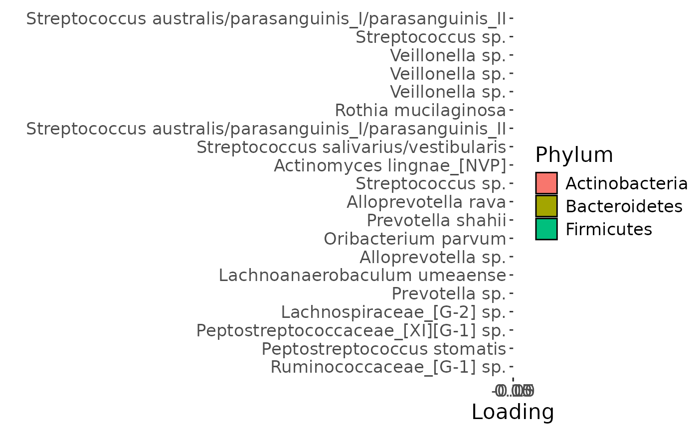
b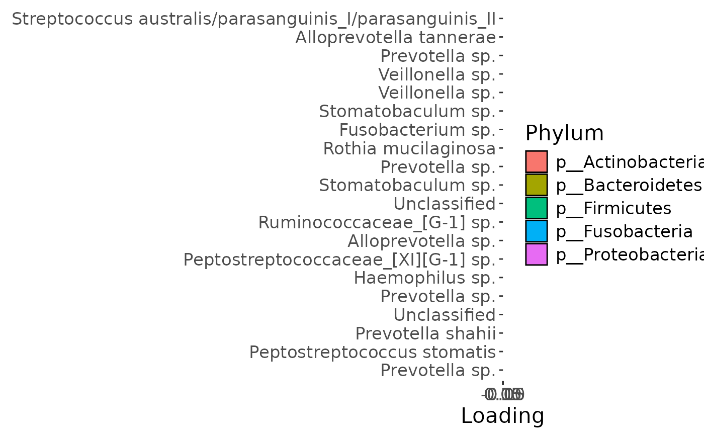
c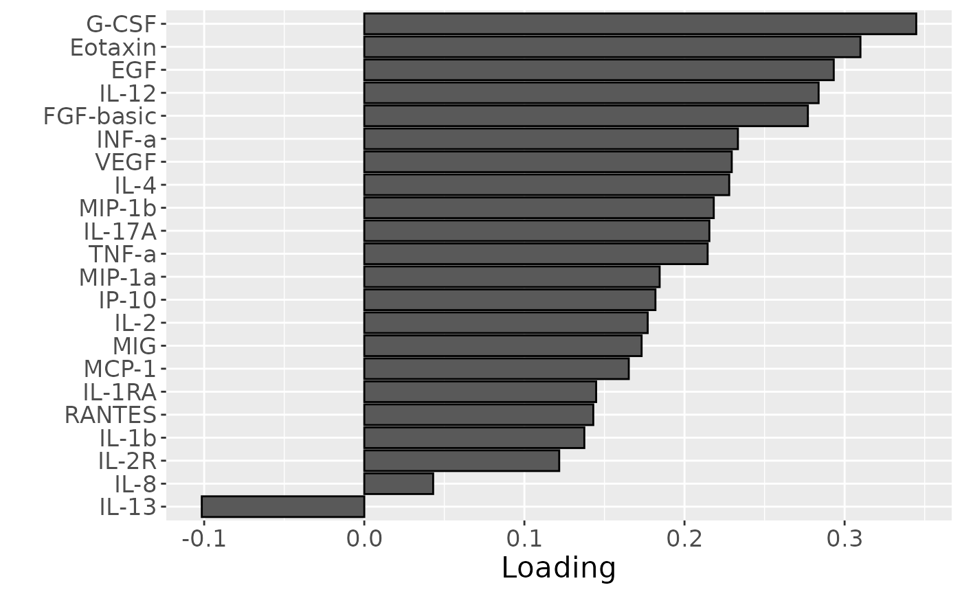
d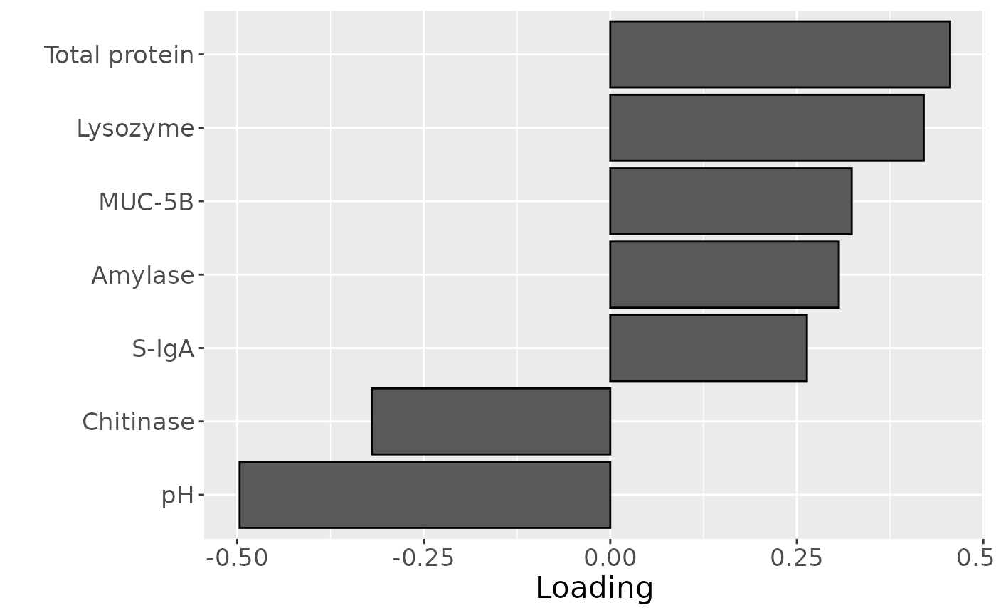
a = acmtf_model$Fac[[3]][,2] %>% as_tibble() %>% mutate(value=-1*value) %>% mutate(timepoint=c(0,3,6,12)) %>% ggplot(aes(x=timepoint,y=value)) + geom_line() + geom_point() + xlab("Time point [months]") + ylab("Loading") + ylim(0,1)

b = acmtf_model$Fac[[5]][,2] %>% as_tibble() %>% mutate(value=-1*value) %>% mutate(timepoint=c(0,3,6,12)) %>% ggplot(aes(x=timepoint,y=value)) + geom_line() + geom_point() + xlab("Time point [months]") + ylab("Loading") + ylim(0,1)

c = acmtf_model$Fac[[7]][,2] %>% as_tibble() %>% mutate(value=-1*value) %>% mutate(timepoint=c(0,3,12)) %>% ggplot(aes(x=timepoint,y=value)) + geom_line() + geom_point() + xlab("Time point [months]") + ylab("Loading") + ylim(-1,1)

d = acmtf_model$Fac[[9]][,2] %>% as_tibble() %>% mutate(value=value) %>% mutate(timepoint=c(0,3,6,12)) %>% ggplot(aes(x=timepoint,y=value)) + geom_line() + geom_point() + xlab("Time point [months]") + ylab("Loading") + ylim(0,1)

a
b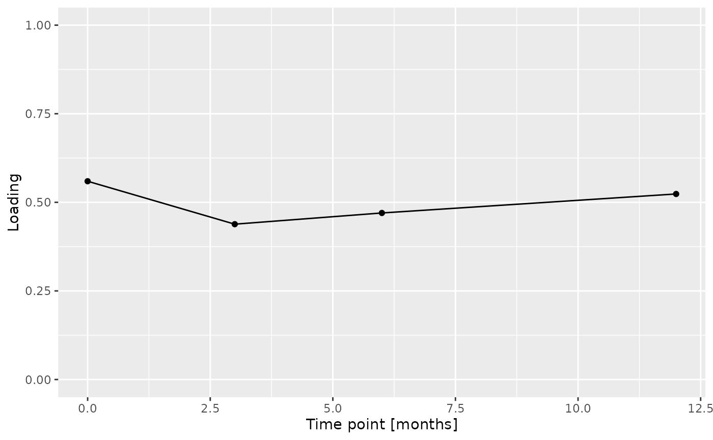
c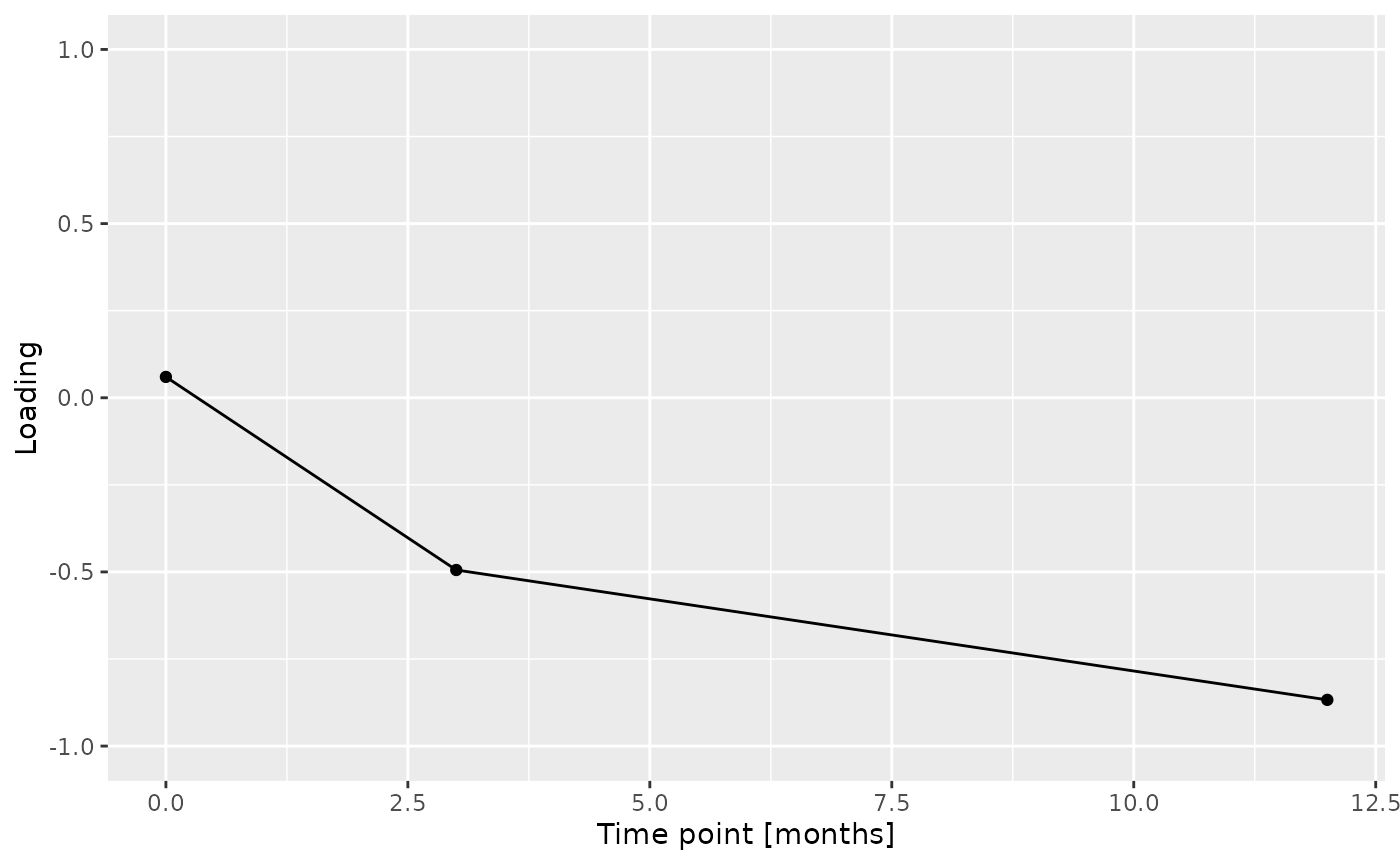
d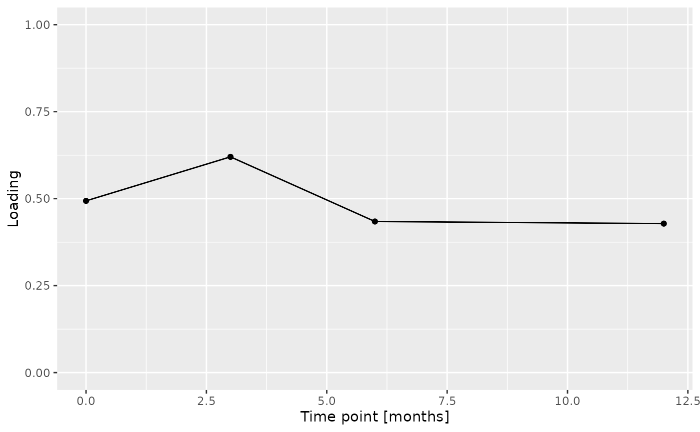
ACMTF-R
Processing
deltaT = NPLStoolbox::Cornejo2025$Circulatory_hormones$data[,1,2] - NPLStoolbox::Cornejo2025$Circulatory_hormones$data[,1,1]
outcome = NPLStoolbox::Cornejo2025$Circulatory_hormones$mode1 %>% mutate(deltaT = deltaT) %>% filter(deltaT != "NA")

homogenizedSamples1 = intersect(NPLStoolbox::Cornejo2025$Tongue_microbiome$mode1$subject, outcome$subject)
homogenizedSamples2 = intersect(NPLStoolbox::Cornejo2025$Salivary_microbiome$mode1$subject, outcome$subject)
homogenizedSamples3 = intersect(NPLStoolbox::Cornejo2025$Salivary_cytokines$mode1$subject, outcome$subject)
homogenizedSamples4 = intersect(NPLStoolbox::Cornejo2025$Salivary_biochemistry$mode1$subject, outcome$subject)

homogenizedSamples = intersect(intersect(homogenizedSamples1, homogenizedSamples2), intersect(homogenizedSamples3,homogenizedSamples4))

outcome = outcome %>% filter(subject %in% homogenizedSamples)

# Tongue
newTongue = NPLStoolbox::Cornejo2025$Tongue

mask = newTongue$mode1$subject %in% homogenizedSamples
newTongue$data = newTongue$data[mask,,]
newTongue$mode1 = newTongue$mode1[mask,]

processedTongue = processDataCube(newTongue, sparsityThreshold = 0.5, considerGroups=TRUE, groupVariable="GenderID", CLR=TRUE, centerMode=1, scaleMode=2)

# Saliva
newSaliva = NPLStoolbox::Cornejo2025$Salivary_microbiome

mask = newSaliva$mode1$subject %in% homogenizedSamples
newSaliva$data = newSaliva$data[mask,,]
newSaliva$mode1 = newSaliva$mode1[mask,]

processedSaliva = processDataCube(newSaliva, sparsityThreshold = 0.5, considerGroups=TRUE, groupVariable="GenderID", CLR=TRUE, centerMode=1, scaleMode=2)

# Cytokines
newCytokines = NPLStoolbox::Cornejo2025$Salivary_cytokines

mask = newCytokines$mode1$subject %in% homogenizedSamples
newCytokines$data = log(newCytokines$data[mask,,] + 0.1300)
newCytokines$mode1 = newCytokines$mode1[mask,]

processedCytokines = processDataCube(newCytokines, CLR=FALSE, centerMode=1, scaleMode=2)

# Biochemistry
newBio = NPLStoolbox::Cornejo2025$Salivary_biochemistry

mask = newBio$mode1$subject %in% homogenizedSamples
newBio$data = log(newBio$data[mask,,])
newBio$mode1 = newBio$mode1[mask,]

processedBiochemistry = processDataCube(newBio, CLR=FALSE, centerMode=1, scaleMode=2)

# Prep data
datasets = list(processedTongue$data, processedSaliva$data, processedCytokines$data, processedBiochemistry$data)
modes = list(c(1,2,3),c(1,4,5),c(1,6,7),c(1,8,9))
Z = setupCMTFdata(datasets, modes, normalize=TRUE)

Y = as.matrix(outcome$deltaT)
Ycnt = Y - mean(Y)
Ynorm = Ycnt / norm(Ycnt, "2")
Model selection
# Please see the separate R scripts at https://doi.org/10.5281/zenodo.16993009 for the model selection.
acmtfr_model90 = readRDS("./GOHTRANS/GOHTRANS_ACMTFR_model_90_deltaT.RDS")
acmtfr_model90$varExp
#> [1] 11.75326 10.52592 48.49405 21.44593
Description
ACMTF-R was applied to supervise the joint decomposition using the difference in free testosterone between baseline and month three of GAHT as dependent variable (y). The model selection procedure revealed that two components were appropriate for all tested pi values, based on a low degeneracy score and RMSECV minimum. Subsequently, the two-component ACMTF-R model using pi=0.90 was selected for further interpretation due to balancing explaining the independent data and predicting y. The model explained 11.8%, 10.5%, 48.5%, 21.4%, and 21.2%, of the variation in the tongue microbiome, salivary microbiome, salivary cytokine, salivary biochemistry, and y, respectively.
The Lambda-matrix of the model revealed that the first component was distinct to the salivary cytokine block, while the second component was common with a slightly larger contribution from the salivary biochemistry block compared to the other blocks. MLR analysis revealed that the first component captured uninterpretable variation, while the second component was exclusively associated with gender identity. The second component was further inspected.
testMetadata(acmtfr_model90, 1, processedTongue)
#> Joining with `by = join_by(subject, GenderID)`
#>       Term    Estimate                                       CI    P_value
#> 1 GenderID  107.196454  -0.0878380361799178 – 0.302230943724517 0.26223444
#> 2      Age    1.032685 -0.0205386077434815 – 0.0226039782431669 0.92072939
#> 3      BOP   -3.139316  -0.0171356225316767 – 0.010856990431065 0.64207341
#> 4     CODS -183.313346  -0.402449852187934 – 0.0358231592929213 0.09553443
#> 5       XI   -4.486779 -0.0274693780964974 – 0.0184958199200182 0.68556771
#>    P_adjust
#> 1 0.6555861
#> 2 0.9207294
#> 3 0.8569596
#> 4 0.4776721
#> 5 0.8569596
testMetadata(acmtfr_model90, 2, processedTongue)
#> Joining with `by = join_by(subject, GenderID)`
#>       Term    Estimate                                        CI     P_value
#> 1 GenderID  266.221675    0.0878259947951316 – 0.444617355260422 0.005861852
#> 2      Age    4.822009  -0.0149089909479829 – 0.0245530087012541 0.612765535
#> 3      BOP    2.819804 -0.00998244764429835 – 0.0156220556012605 0.648039386
#> 4     CODS -115.152380    -0.31559388121747 – 0.0852891217318665 0.242060921
#> 5       XI   -6.577535  -0.0275994394345139 – 0.0144443691718177 0.518009580
#>     P_adjust
#> 1 0.02930926
#> 2 0.64803939
#> 3 0.64803939
#> 4 0.60515230
#> 5 0.64803939
lambda = abs(acmtfr_model90$Fac[[10]])
colnames(lambda) = paste0("C", 1:2)

lambda %>%
  as_tibble() %>%
  mutate(block=c("tongue", "saliva", "cytokines", "biochemistry")) %>%
  mutate(block=factor(block, levels=c("tongue", "saliva", "cytokines", "biochemistry"))) %>%
  pivot_longer(-block) %>%
  ggplot(aes(x=as.factor(name),y=value,fill=as.factor(block))) +
  geom_bar(stat="identity",position=position_dodge(),col="black") +
  xlab("ACMTF-R component number") +
  ylab(expression(lambda)) +
  scale_x_discrete(labels=1:3) +
  scale_fill_manual(name="Dataset",values = hue_pal()(5),labels=c("Tongue microbiome", "Salivary microbiome", "Salivary cytokines", "Salivary biochemistry")) +
  theme(legend.position="top")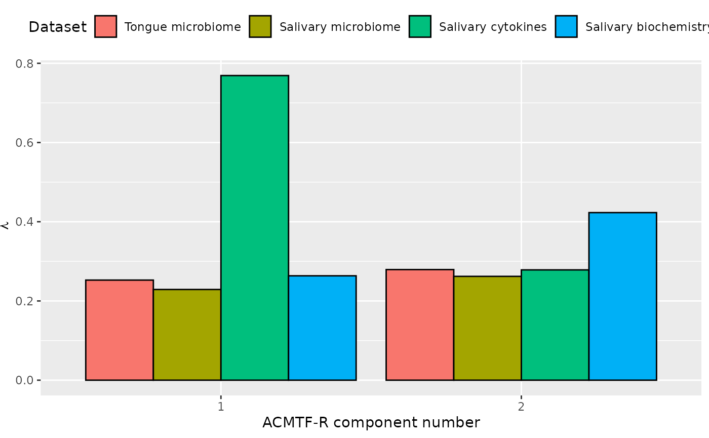
# Tongue
topIndices = processedTongue$mode2 %>% mutate(index=1:nrow(.), Comp = acmtfr_model90$Fac[[2]][,2]) %>% arrange(desc(Comp)) %>% head() %>% select(index) %>% pull()
bottomIndices = processedTongue$mode2 %>% mutate(index=1:nrow(.), Comp = acmtfr_model90$Fac[[2]][,2]) %>% arrange(desc(Comp)) %>% tail() %>% select(index) %>% pull()

Xhat = parafac4microbiome::reinflateTensor(acmtfr_model90$Fac[[1]][,2], acmtf_model$Fac[[2]][,2], acmtf_model$Fac[[3]][,2])

cor(Xhat[,topIndices[1],], Ynorm) # flip
#>          [,1]
#> [1,] 0.460004
#> [2,] 0.460004
#> [3,] 0.460004
#> [4,] 0.460004
cor(Xhat[,bottomIndices[6],], Ynorm)
#>           [,1]
#> [1,] -0.460004
#> [2,] -0.460004
#> [3,] -0.460004
#> [4,] -0.460004

# Saliva
topIndices = processedSaliva$mode2 %>% mutate(index=1:nrow(.), Comp = acmtfr_model90$Fac[[4]][,2]) %>% arrange(desc(Comp)) %>% head() %>% select(index) %>% pull()
bottomIndices = processedSaliva$mode2 %>% mutate(index=1:nrow(.), Comp = acmtfr_model90$Fac[[4]][,2]) %>% arrange(desc(Comp)) %>% tail() %>% select(index) %>% pull()

Xhat = parafac4microbiome::reinflateTensor(acmtfr_model90$Fac[[1]][,2], acmtfr_model90$Fac[[4]][,2], acmtfr_model90$Fac[[5]][,2])

cor(Xhat[,topIndices[1],], Ynorm) # no flip
#>          [,1]
#> [1,] 0.460004
#> [2,] 0.460004
#> [3,] 0.460004
#> [4,] 0.460004
cor(Xhat[,bottomIndices[6],], Ynorm)
#>           [,1]
#> [1,] -0.460004
#> [2,] -0.460004
#> [3,] -0.460004
#> [4,] -0.460004

# Cytokines
topIndices = processedCytokines$mode2 %>% mutate(index=1:nrow(.), Comp = acmtfr_model90$Fac[[6]][,2]) %>% arrange(desc(Comp)) %>% head() %>% select(index) %>% pull()
bottomIndices = processedCytokines$mode2 %>% mutate(index=1:nrow(.), Comp = acmtfr_model90$Fac[[6]][,2]) %>% arrange(desc(Comp)) %>% tail() %>% select(index) %>% pull()

Xhat = parafac4microbiome::reinflateTensor(acmtfr_model90$Fac[[1]][,2], acmtfr_model90$Fac[[6]][,2], acmtfr_model90$Fac[[7]][,2])

cor(Xhat[,topIndices[1],], Ynorm) # no flip
#>           [,1]
#> [1,] -0.460004
#> [2,]  0.460004
#> [3,]  0.460004
cor(Xhat[,bottomIndices[6],], Ynorm)
#>           [,1]
#> [1,]  0.460004
#> [2,] -0.460004
#> [3,] -0.460004

# Biochemistry
topIndices = 7
bottomIndices = 1

Xhat = parafac4microbiome::reinflateTensor(acmtfr_model90$Fac[[1]][,2], acmtfr_model90$Fac[[8]][,2], acmtfr_model90$Fac[[9]][,2])

cor(Xhat[,topIndices,], Ynorm) # no flip
#>          [,1]
#> [1,] 0.460004
#> [2,] 0.460004
#> [3,] 0.460004
#> [4,] 0.460004
cor(Xhat[,bottomIndices,], Ynorm)
#>           [,1]
#> [1,] -0.460004
#> [2,] -0.460004
#> [3,] -0.460004
#> [4,] -0.460004
# Tongue
temp = processedTongue$mode2 %>%
  as_tibble() %>%
  mutate(Component_1 = -1*acmtfr_model90$Fac[[2]][,2]) %>%
  mutate(Genus = gsub("g__", "", Genus), Species = gsub("s__", "", Species)) %>%
  mutate(Species = gsub("\\(", "", Species)) %>%
  mutate(Species = gsub("\\)", "", Species))

fixedSpeciesNames = str_split_fixed(temp$Species, "/", 5) %>%
  as_tibble() %>%
  mutate(dplyr::across(.cols = everything(), .fns = ~ dplyr::if_else(stringr::str_detect(.x, "sp."), "", .x)))
fixedSpeciesNames[fixedSpeciesNames$V1 == "", "V1"] = "sp."
fixedSpeciesNames = fixedSpeciesNames %>%
  mutate(name=paste0(V1, "/", V2)) %>%
  mutate(name=gsub("/$", "", name)) %>%
  mutate(name=paste0(name, "/", V3)) %>%
  mutate(name=gsub("/$", "", name)) %>%
  mutate(name=paste0(name, "/", V4)) %>%
  mutate(name=gsub("/$", "", name)) %>%
  mutate(name=paste0(name, "/", V5)) %>%
  mutate(name=gsub("/$", "", name))

temp$Species = fixedSpeciesNames$name
temp$name = paste0(temp$Genus, " ", temp$Species)
temp[temp$name == " sp.", "name"] = "Unclassified"
temp[temp$name == " ", "name"] = "Unclassified"
temp[temp$name == " sp.", "name"] = "Unclassified"

temp = temp %>%
  arrange(Component_1) %>%
  mutate(index=1:nrow(.)) %>%
  filter(index %in% c(1:10,228:237))

a=temp %>%
  ggplot(aes(x=Component_1,y=as.factor(index),fill=as.factor(Phylum))) +
  geom_bar(stat="identity", col="black") +
  scale_y_discrete(label=temp$name) +
  xlab("Loading") +
  ylab("") +
  scale_fill_manual(name="Phylum", labels=c("Actinobacteria", "Bacteroidetes", "Firmicutes", "Proteobacteria"), values=hue_pal()(5)[-4]) +
  theme(text=element_text(size=16))

# Saliva comp 1
temp = processedSaliva$mode2 %>%
  as_tibble() %>%
  mutate(Component_1 = acmtfr_model90$Fac[[4]][,2]) %>%
  mutate(Genus = gsub("g__", "", Genus), Species = gsub("s__", "", Species)) %>%
  mutate(Species = gsub("\\(", "", Species)) %>%
  mutate(Species = gsub("\\)", "", Species))

fixedSpeciesNames = str_split_fixed(temp$Species, "/", 5) %>%
  as_tibble() %>%
  mutate(dplyr::across(.cols = everything(), .fns = ~ dplyr::if_else(stringr::str_detect(.x, "sp."), "", .x)))
fixedSpeciesNames[fixedSpeciesNames$V1 == "", "V1"] = "sp."
fixedSpeciesNames = fixedSpeciesNames %>%
  mutate(name=paste0(V1, "/", V2)) %>%
  mutate(name=gsub("/$", "", name)) %>%
  mutate(name=paste0(name, "/", V3)) %>%
  mutate(name=gsub("/$", "", name)) %>%
  mutate(name=paste0(name, "/", V4)) %>%
  mutate(name=gsub("/$", "", name)) %>%
  mutate(name=paste0(name, "/", V5)) %>%
  mutate(name=gsub("/$", "", name))

temp$Species = fixedSpeciesNames$name
temp$name = paste0(temp$Genus, " ", temp$Species)
temp[temp$name == " sp.", "name"] = "Unclassified"
temp[temp$name == " ", "name"] = "Unclassified"
temp[temp$name == " sp.", "name"] = "Unclassified"

temp = temp %>%
  arrange(Component_1) %>%
  mutate(index=1:nrow(.)) %>%
  filter(index %in% c(1:10,260:269))

b=temp %>%
  ggplot(aes(x=Component_1,y=as.factor(index),fill=as.factor(Phylum))) +
  geom_bar(stat="identity", col="black") +
  scale_y_discrete(label=temp$name) +
  xlab("Loading") +
  ylab("") +
  guides(fill=guide_legend(title="Phylum")) +
  theme(text=element_text(size=16))

# Cytokines
temp = processedCytokines$mode2 %>%
  mutate(Comp = acmtfr_model90$Fac[[6]][,2]) %>%
  arrange(Comp) %>%
  mutate(index=1:nrow(.)) %>%
  mutate(V1 = gsub("_pg_ml", "", V1)) %>%
  mutate(V1 = gsub("_", "-", V1))

c = temp %>%
  ggplot(aes(x=Comp,y=as.factor(index))) +
  geom_bar(stat="identity", col="black") +
  xlab("Loading") +
  ylab("") +
  scale_y_discrete(labels=temp$V1) +
  theme(text=element_text(size=16))

# Biochemistry comp 1
temp = processedBiochemistry$mode2 %>%
  mutate(Comp = acmtfr_model90$Fac[[8]][,2]) %>%
  arrange(Comp) %>%
  mutate(index=1:nrow(.)) %>%
  mutate(V1 = c("pH", "Chitinase", "S-IgA", "MUC-5B", "Amylase", "Lysozyme", "Total protein"))

d = temp %>%
  ggplot(aes(x=Comp,y=as.factor(index))) +
  geom_bar(stat="identity", col="black") +
  xlab("Loading") +
  ylab("") +
  scale_y_discrete(labels=temp$V1) +
  theme(text=element_text(size=16))

a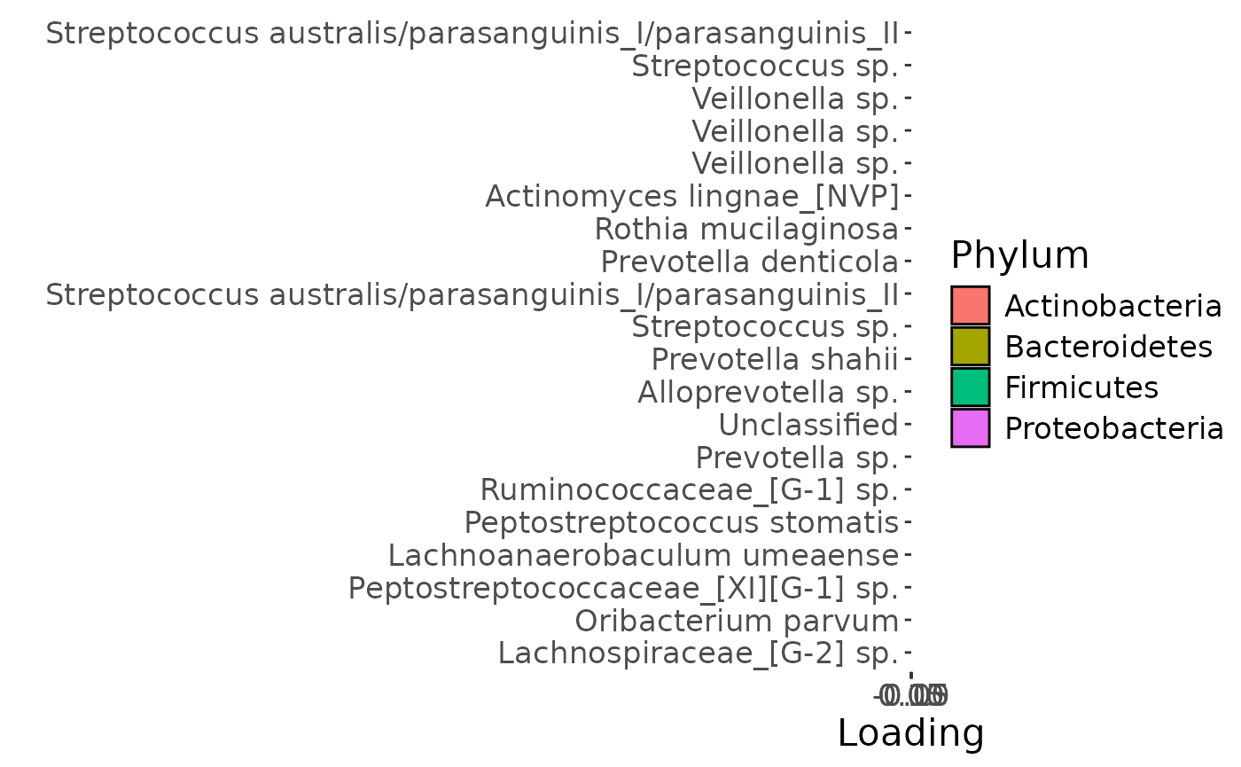
b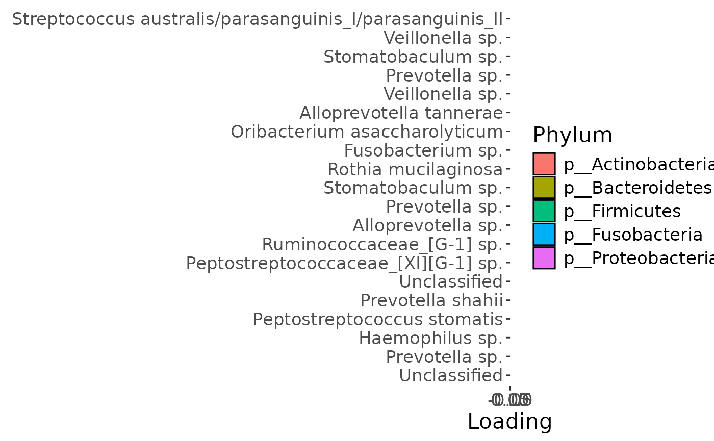
c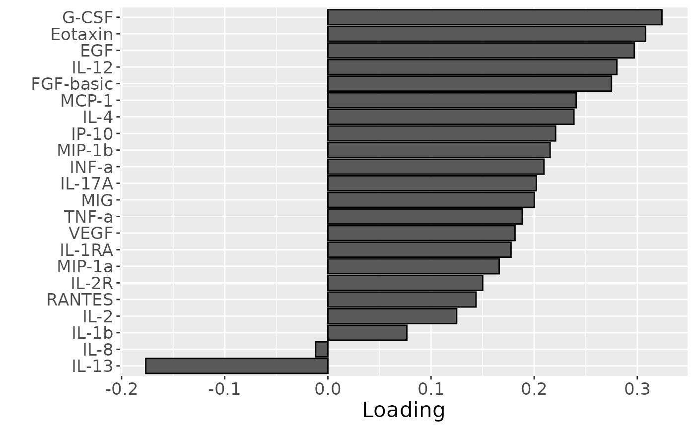
d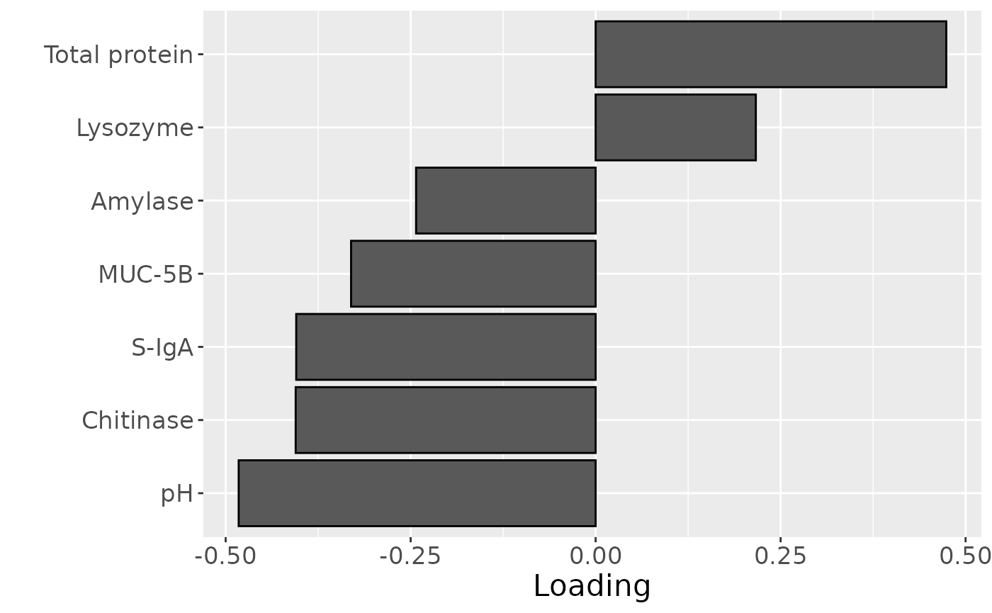
a = acmtfr_model90$Fac[[3]][,2] %>% as_tibble() %>% mutate(value=-1*value) %>% mutate(timepoint=c(0,3,6,12)) %>% ggplot(aes(x=timepoint,y=value)) + geom_line() + geom_point() + xlab("Time point [months]") + ylab("Loading") + ylim(0,1)

b = acmtfr_model90$Fac[[5]][,2] %>% as_tibble() %>% mutate(value=-1*value) %>% mutate(timepoint=c(0,3,6,12)) %>% ggplot(aes(x=timepoint,y=value)) + geom_line() + geom_point() + xlab("Time point [months]") + ylab("Loading") + ylim(0,1)

c = acmtfr_model90$Fac[[7]][,2] %>% as_tibble() %>% mutate(value=-1*value) %>% mutate(timepoint=c(0,3,12)) %>% ggplot(aes(x=timepoint,y=value)) + geom_line() + geom_point() + xlab("Time point [months]") + ylab("Loading") + ylim(-1,1)

d = acmtfr_model90$Fac[[9]][,2] %>% as_tibble() %>% mutate(value=-1*value) %>% mutate(timepoint=c(0,3,6,12)) %>% ggplot(aes(x=timepoint,y=value)) + geom_line() + geom_point() + xlab("Time point [months]") + ylab("Loading") + ylim(0,1)

a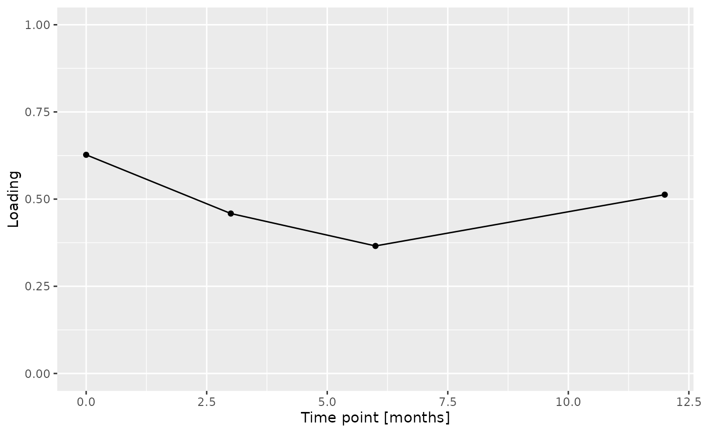
b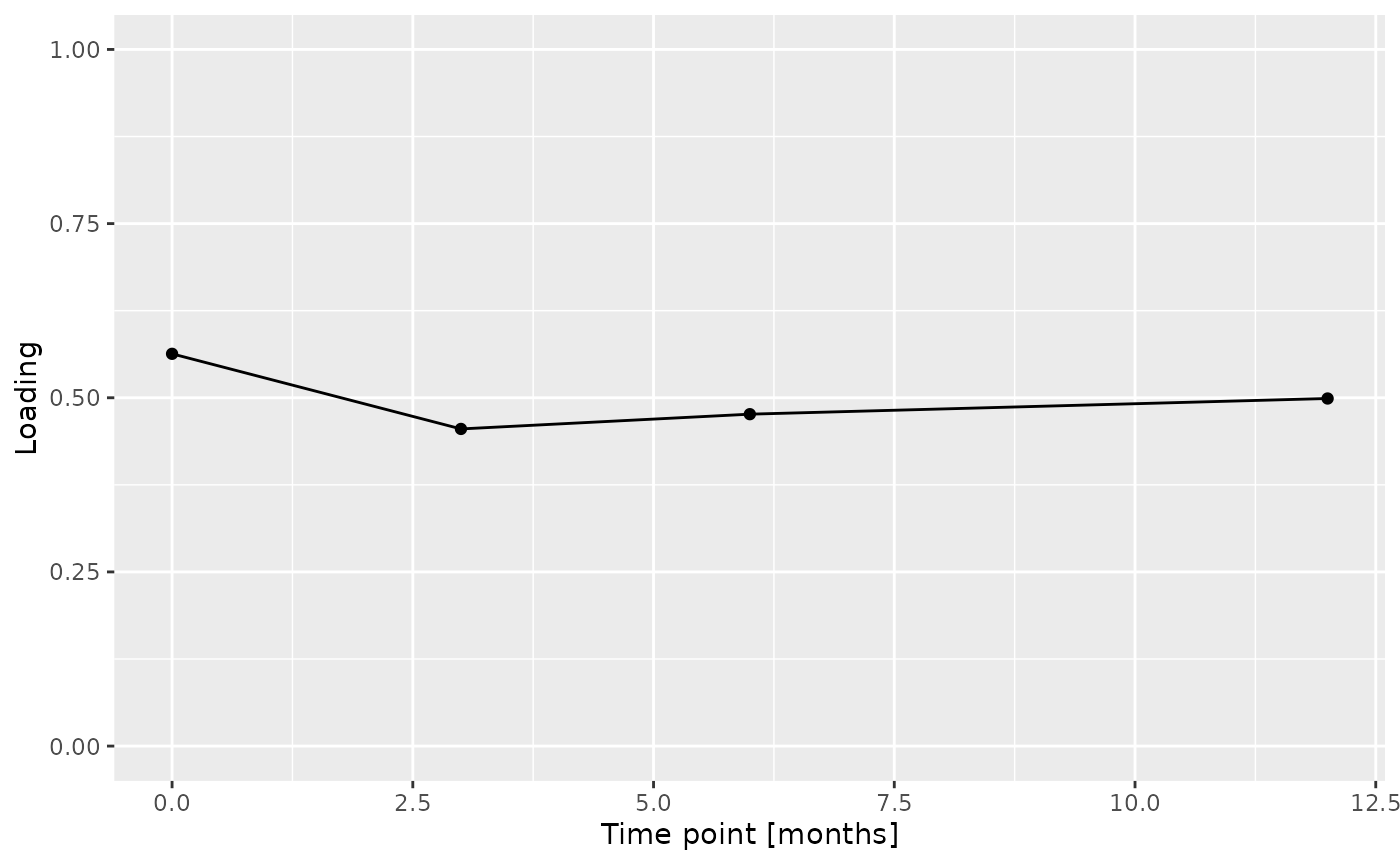
c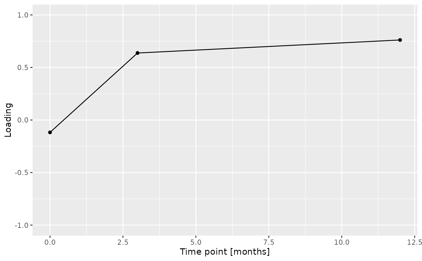
d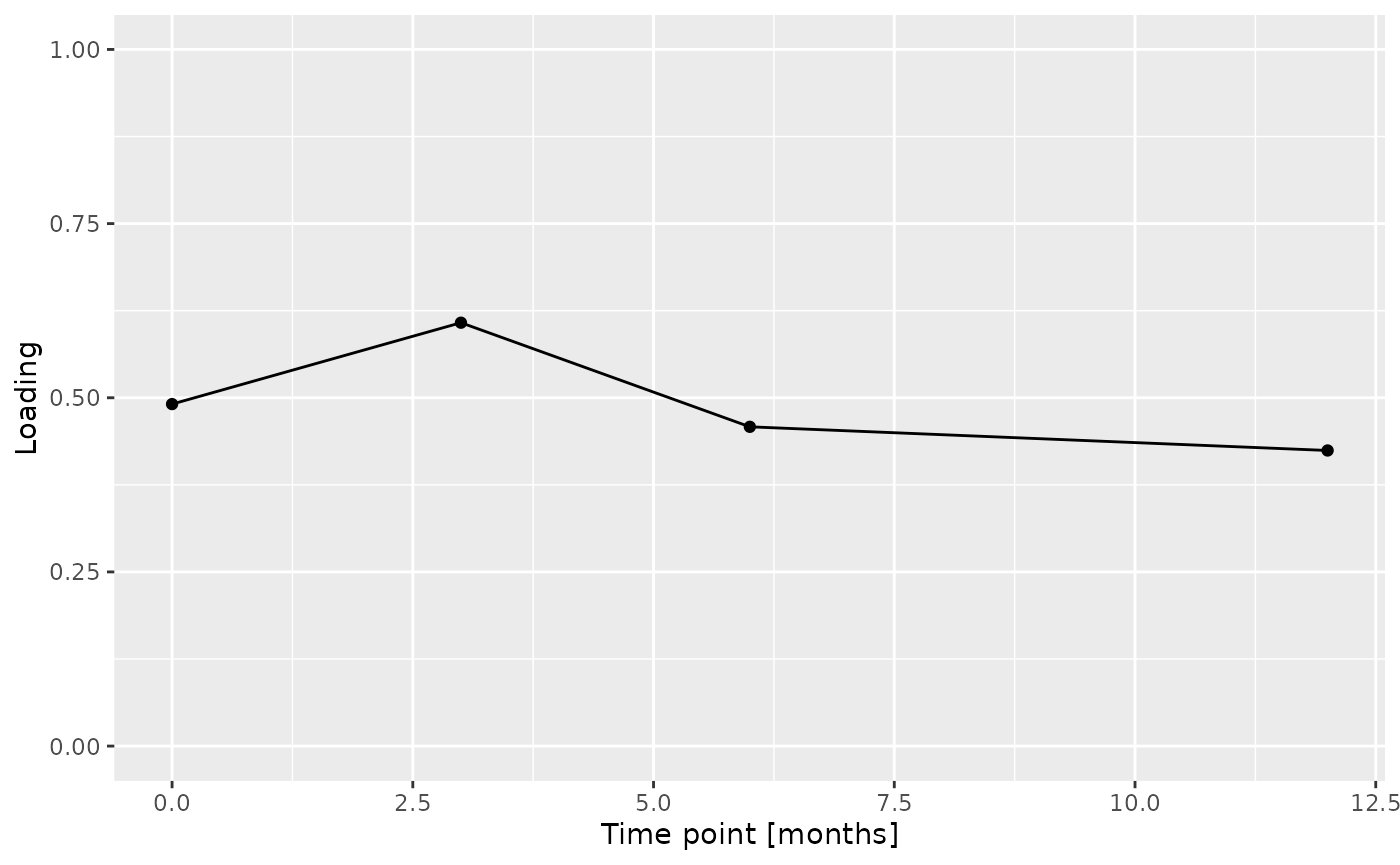
Positively loaded microbiota in the tongue microbiome including Streptococcus australis / parasanguinis, Streptococcus spp., Veillonella spp., Actinomyces lingae, Rothia mucilaginosa, and Prevotella denticola were enriched in transfeminine participants and depleted in transmasculine participants. Conversely, negatively microbiota including Lachnospiraceae sp., Oribacterium parvum, Peptostreptococcaceae sp., Lachnoanaerobaculum umeaense, Peptostreptococcus stomatis, Ruminococcaceae sp., Prevotella sp., Alloprevotella sp., and Prevotella shahii were enriched in transmasculine participants and depleted in transfeminine participants. The time mode loadings indicate that inter-subject differences due to GAHT decreased over time.
Positively loaded microbiota in the salivary microbiome including Streptococcus australis / parasanguinis, Veillonella spp., Stomatobaculum spp., Prevotella sp., Alloprevotella tannerae, Oribacterium asaccharolyticum, Fusobacterium sp., and Rothia mucilaginosa were enriched in transfeminine participants and depleted in transmasculine participants. Conversely, negatively loaded microbiota including Prevotella spp., Haemophilus sp., Peptostreptococcus stomatis, Prevotella shahii, Peptostreptococcaceae sp., Ruminococcaceae sp., Alloprevotella sp., and two unclassified ASVs were enriched in transmasculine participants and depleted in transfeminine participants. The time mode loadings indicate that inter-subject differences due to GAHT was stable over time.
Almost all salivary cytokines were positively loaded, indicating that they had higher levels in transfeminine participants and lower levels in transmasculine participants. The exception was IL-13, which had higher levels in transmasculine participants and lower levels in transfeminine participants. The time mode loadings indicate that inter-subject differences due to GAHT were absent at baseline and constant thereafter.
Total protein and lysozyme levels were positively loaded for the salivary biochemistry block, indicating higher levels in transfeminine participants and lower levels in transmasculine participants. pH, chitinase, S-IgA, MUC-5B, and amylase were negatively loaded, indicating higher levels in transmasculine participants and lower levels in transfeminine participants. The time mode loadings indicate that these differences mainly occurred after three months of GAHT.