MAINHEALTH: intergenerational obesity transmission
2025-08-31
Source:vignettes/articles/MAINHEALTH.Rmd
MAINHEALTH.RmdPreamble
testMetadata = function(model, comp, metadata){
  transformedSubjectLoadings = model$Fac[[1]][,comp]
  transformedSubjectLoadings = transformedSubjectLoadings / norm(transformedSubjectLoadings, "2")

  result = lm(transformedSubjectLoadings ~ BMI + C.section + Secretor + Lewis + whz.6m, data=metadata$mode1)

  # Extract coefficients and confidence intervals
  coef_estimates <- summary(result)$coefficients
  conf_intervals <- confint(result)

  # Remove intercept
  coef_estimates <- coef_estimates[rownames(coef_estimates) != "(Intercept)", ]
  conf_intervals <- conf_intervals[rownames(conf_intervals) != "(Intercept)", ]

  # Combine into a clean data frame
  summary_table <- data.frame(
    Term     = rownames(coef_estimates),
    Estimate = coef_estimates[, "Estimate"] * 1e3,
    CI       = paste0(
                 conf_intervals[, 1], " – ",
                 conf_intervals[, 2]
               ),
    P_value  = coef_estimates[, "Pr(>|t|)"],
    P_adjust = p.adjust(coef_estimates[, "Pr(>|t|)"], "BH"),
    row.names = NULL
  )

  return(summary_table)
}
# Old approach
# Needed colours: BMI groups (3) and phyla levels (6)
# colours = hue_pal()(9)
# #show_col(colours)
# BMI_cols = colours[c(1,4,7)]
# phylum_cols = colours[-c(1,4,7)]

# Rasmus's suggestion
colours = RColorBrewer:: brewer.pal(8, "Dark2")
BMI_cols = c("darkgreen","darkgoldenrod","darkred") #colours[1:3]
WHZ_cols = c("darkgreen", "darkgoldenrod", "dodgerblue4")
phylum_cols = colours
ACMTF
Processing
homogenizedSamples = intersect(intersect(NPLStoolbox::Jakobsen2025$faeces$mode1 %>% filter(!is.na(BMI)) %>% select(subject) %>% pull(), NPLStoolbox::Jakobsen2025$milkMicrobiome$mode1 %>% filter(!is.na(BMI)) %>% select(subject) %>% pull()), NPLStoolbox::Jakobsen2025$milkMetabolomics$mode1 %>% filter(!is.na(BMI)) %>% select(subject) %>% pull())

# Faeces
newFaeces = NPLStoolbox::Jakobsen2025$faeces

mask = newFaeces$mode1$subject %in% homogenizedSamples
newFaeces$data = newFaeces$data[mask,,]
newFaeces$mode1 = newFaeces$mode1[mask,]
processedFaeces = parafac4microbiome::processDataCube(newFaeces, sparsityThreshold = 0.75, centerMode=1, scaleMode=2)

# Milk
newMilk = NPLStoolbox::Jakobsen2025$milkMicrobiome

mask = newMilk$mode1$subject %in% homogenizedSamples
newMilk$data = newMilk$data[mask,,]
newMilk$mode1 = newMilk$mode1[mask,]
processedMilk = parafac4microbiome::processDataCube(newMilk, sparsityThreshold=0.85, centerMode=1, scaleMode=2)

# Milk metab
newMilkMetab = NPLStoolbox::Jakobsen2025$milkMetabolomics

mask = newMilkMetab$mode1$subject %in% homogenizedSamples
newMilkMetab$data = newMilkMetab$data[mask,,]
newMilkMetab$mode1 = newMilkMetab$mode1[mask,]
processedMilkMetab = parafac4microbiome::processDataCube(newMilkMetab, CLR=FALSE, centerMode=1, scaleMode=2)

datasets = list(processedFaeces$data, processedMilk$data, processedMilkMetab$data)
modes = list(c(1,2,3), c(1,4,5), c(1,6,7))
Z = setupCMTFdata(datasets, modes, normalize=TRUE)
Model selection
# Please see the separate R scripts at https://doi.org/10.5281/zenodo.16993009 for the model selection.
model_ACMTF = readRDS("./MAINHEALTH/ACMTF_model_bmi.RDS")
model_ACMTF$varExp
#> [1] 14.25607 10.22240  5.99588
Description
ACMTF was applied to capture to dominant source of variation across all data blocks. The model selection procedure revealed that FMS CV dropped below 0.9 when three components were selected. Therefore, a two-component ACMTF model was selected, explaining 14.3%, 10.2%, 6.0% of variation in the infant faecal microbiome, HM microbiome, and HM metabolomics data blocks, respectively. The Lambda-matrix of the model revealed that the first component was predominantly distinct to the infant faecal microbiome data block, while the second was local to the infant faecal and HM microbiome blocks. However, MLR analysis revealed that the first and second component captured variation associated with a mixture of maternal ppBMI and maternal secretor status.
testMetadata(model_ACMTF, 1, processedFaeces)
#>        Term   Estimate                                           CI
#> 1       BMI  -2.276732 -0.00450781299767528 – -4.56503944847972e-05
#> 2 C.section   4.715650      -0.0361024191316937 – 0.045533718733486
#> 3  Secretor -84.617925     -0.112828298007938 – -0.0564075514364901
#> 4     Lewis  55.837894        -0.024014950520992 – 0.13569073945265
#> 5    whz.6m   3.157397     -0.0075259356824812 – 0.0138407294998676
#>        P_value     P_adjust
#> 1 4.556168e-02 1.139042e-01
#> 2 8.195074e-01 8.195074e-01
#> 3 2.717526e-08 1.358763e-07
#> 4 1.688349e-01 2.813915e-01
#> 5 5.596344e-01 6.995429e-01
testMetadata(model_ACMTF, 2, processedFaeces)
#>        Term    Estimate                                         CI      P_value
#> 1       BMI  -4.4150025 -0.00694585174854792 – -0.0018841532867865 0.0007595475
#> 2 C.section -40.0909098  -0.0863932916037776 – 0.00621147209552562 0.0890716786
#> 3  Secretor  41.3042948    0.0093035776930651 – 0.0733050118693837 0.0118369347
#> 4     Lewis  72.2848185    -0.0182970492398522 – 0.162866686186581 0.1167744722
#> 5    whz.6m   0.9816376   -0.0111371068252218 – 0.0131003820123962 0.8728860770
#>      P_adjust
#> 1 0.003797738
#> 2 0.145968090
#> 3 0.029592337
#> 4 0.145968090
#> 5 0.872886077
lambda = abs(model_ACMTF$Fac[[8]])
colnames(lambda) = paste0("C", 1:2)

lambda %>%
  as_tibble() %>%
  mutate(block=c("Infant faecal microbiome", "HM microbiome", "HM metabolome")) %>%
  # mutate(block=factor(block, levels=c("tongue", "lowling", "lowinter", "upling", "upinter", "saliva", "metab"))) %>%
  pivot_longer(-block) %>%
  ggplot(aes(x=as.factor(name),y=value,fill=as.factor(block))) +
  geom_bar(stat="identity",position=position_dodge(),col="black") +
  xlab("ACMTF component number") +
  ylab(expression(lambda)) +
  scale_x_discrete(labels=1:3) +
  scale_fill_manual(name="Dataset",values = hue_pal()(3),labels=c("HM metabolome", "HM microbiome", "Infant faecal microbiome")) +
  theme(legend.position="top", text=element_text(size=16))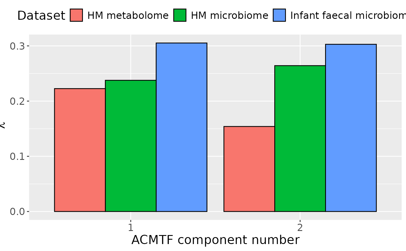
# Faeces
topIndices = processedFaeces$mode2 %>% mutate(index=1:nrow(.), Comp = model_ACMTF$Fac[[2]][,1]) %>% arrange(desc(Comp)) %>% head() %>% select(index) %>% pull()
bottomIndices = processedFaeces$mode2 %>% mutate(index=1:nrow(.), Comp = model_ACMTF$Fac[[2]][,1]) %>% arrange(desc(Comp)) %>% tail() %>% select(index) %>% pull()

Xhat = parafac4microbiome::reinflateTensor(model_ACMTF$Fac[[1]][,1], model_ACMTF$Fac[[2]][,1], model_ACMTF$Fac[[3]][,1])

print("Positive loadings:")
#> [1] "Positive loadings:"
print(cor(Xhat[,topIndices[1],1], processedMilkMetab$mode1$Secretor)) # no flip
#> [1] 0.4992547
print("Negative loadings:")
#> [1] "Negative loadings:"
print(cor(Xhat[,bottomIndices[1],1], processedMilkMetab$mode1$Secretor))
#> [1] -0.4992547

print("Positive loadings:")
#> [1] "Positive loadings:"
print(cor(Xhat[,topIndices[1],1], processedMilkMetab$mode1$BMI)) # no flip
#> [1] 0.07586748
print("Negative loadings:")
#> [1] "Negative loadings:"
print(cor(Xhat[,bottomIndices[1],1], processedMilkMetab$mode1$BMI))
#> [1] -0.07586748

# Milk
topIndices = processedMilk$mode2 %>% mutate(index=1:nrow(.), Comp = model_ACMTF$Fac[[4]][,1]) %>% arrange(desc(Comp)) %>% head() %>% select(index) %>% pull()
bottomIndices = processedMilk$mode2 %>% mutate(index=1:nrow(.), Comp = model_ACMTF$Fac[[4]][,1]) %>% arrange(desc(Comp)) %>% tail() %>% select(index) %>% pull()

Xhat = 1 * parafac4microbiome::reinflateTensor(model_ACMTF$Fac[[1]][,1], model_ACMTF$Fac[[4]][,1], model_ACMTF$Fac[[5]][,1])

print("Positive loadings:")
#> [1] "Positive loadings:"
print(cor(Xhat[,topIndices[1],1], processedMilk$mode1$Secretor)) # no flip
#> [1] 0.5156076
print("Negative loadings:")
#> [1] "Negative loadings:"
print(cor(Xhat[,bottomIndices[1],1], processedMilk$mode1$Secretor))
#> [1] -0.5156076

print("Positive loadings:")
#> [1] "Positive loadings:"
print(cor(Xhat[,topIndices[1],1], processedMilk$mode1$BMI)) # no flip
#> [1] 0.07586744
print("Negative loadings:")
#> [1] "Negative loadings:"
print(cor(Xhat[,bottomIndices[1],1], processedMilk$mode1$BMI))
#> [1] -0.07586744

# Milk metab
topIndices = processedMilkMetab$mode2 %>% mutate(index=1:nrow(.), Comp = model_ACMTF$Fac[[6]][,1]) %>% arrange(desc(Comp)) %>% head() %>% select(index) %>% pull()
bottomIndices = processedMilkMetab$mode2 %>% mutate(index=1:nrow(.), Comp = model_ACMTF$Fac[[6]][,1]) %>% arrange(desc(Comp)) %>% tail() %>% select(index) %>% pull()

Xhat = parafac4microbiome::reinflateTensor(model_ACMTF$Fac[[1]][,1], model_ACMTF$Fac[[6]][,1], model_ACMTF$Fac[[7]][,1])

print("Positive loadings:")
#> [1] "Positive loadings:"
print(cor(Xhat[,topIndices[1],1], processedMilkMetab$mode1$Secretor)) # no flip
#> [1] 0.4992547
print("Negative loadings:")
#> [1] "Negative loadings:"
print(cor(Xhat[,bottomIndices[1],1], processedMilkMetab$mode1$Secretor))
#> [1] -0.4992547

print("Positive loadings:")
#> [1] "Positive loadings:"
print(cor(Xhat[,topIndices[1],1], processedMilkMetab$mode1$BMI)) # no flip
#> [1] 0.07586748
print("Negative loadings:")
#> [1] "Negative loadings:"
print(cor(Xhat[,bottomIndices[1],1], processedMilkMetab$mode1$BMI))
#> [1] -0.07586748
a = processedMilk$mode1 %>%
  mutate(Component_1 = model_ACMTF$Fac[[1]][,1]) %>%
  ggplot(aes(x=as.factor(Secretor),y=Component_1)) +
  geom_boxplot() +
  stat_compare_means(comparisons=list(c("0","1")), label="p.signif") +
  xlab("Secretor status") +
  ylab("Loading") +
  scale_x_discrete(labels=c("Se-", "Se+")) +
  theme(text=element_text(size=16))

df = processedFaeces$mode2 %>%
  mutate(Component_1 = model_ACMTF$Fac[[2]][,1]) %>%
  arrange(Component_1) %>%
  mutate(index=1:nrow(.)) %>%
  mutate(Genus = gsub("g__", "", V7), Species = gsub("s__", "", V8)) %>%
  mutate(Species = str_split_fixed(Species, "_", 2)[,2]) %>%
  mutate(dplyr::across(.cols = Species, .fns = ~ dplyr::if_else(stringr::str_detect(.x, "sp."), "", .x))) %>%
  mutate(dplyr::across(.cols = Species, .fns = ~ dplyr::if_else(stringr::str_detect(.x, "organism"), "", .x))) %>%
  mutate(dplyr::across(.cols = Species, .fns = ~ dplyr::if_else(stringr::str_detect(.x, "bacterium"), "", .x))) %>%
  filter(index %in% c(1:10, 84:93))

df[df$Genus == "" & df$Species == "", "Species"] = "Unknown"
df[df$Species == "", "Species"] = "sp."
df$name = paste0(df$Genus, " ", df$Species)

b = df %>%
  ggplot(aes(x=Component_1,y=as.factor(index),fill=as.factor(V3))) +
  geom_bar(stat="identity", col="black") +
  xlab("Loading") +
  ylab("") +
  scale_y_discrete(labels=df$name) +
  scale_fill_manual(name="Phylum", values=hue_pal()(5)[-c(4,5)], labels=c("Actinobacteriota", "Bacteroidota", "Firmicutes")) +
  theme(text=element_text(size=16))

c = model_ACMTF$Fac[[3]][,1] %>%
  as_tibble() %>%
  mutate(value=-1*value) %>%
  ggplot(aes(x=c(30,60,90),y=value)) +
  geom_line() +
  geom_point() +
  xlab("Time point [day]") +
  ylab("Loading") +
  ylim(0,1) +
  theme(text=element_text(size=16))

df = processedMilk$mode2 %>%
  mutate(Component_1 = model_ACMTF$Fac[[4]][,1]) %>%
  arrange(Component_1) %>%
  mutate(index=1:nrow(.)) %>%
  mutate(Genus = gsub("g__", "", V7), Species = gsub("s__", "", V8)) %>%
  mutate(Species = str_split_fixed(Species, "_", 2)[,2]) %>%
  mutate(dplyr::across(.cols = Species, .fns = ~ dplyr::if_else(stringr::str_detect(.x, "sp."), "", .x))) %>%
  mutate(dplyr::across(.cols = Species, .fns = ~ dplyr::if_else(stringr::str_detect(.x, "organism"), "", .x))) %>%
  mutate(dplyr::across(.cols = Species, .fns = ~ dplyr::if_else(stringr::str_detect(.x, "bacterium"), "", .x))) %>%
  filter(index %in% c(1:10, 106:115))

df[df$Genus == "" & df$Species == "", "Species"] = "Unknown"
df[df$Species == "", "Species"] = "sp."
df$name = paste0(df$Genus, " ", df$Species)

d = df %>%
  ggplot(aes(x=Component_1,y=as.factor(index),fill=as.factor(V3))) +
  geom_bar(stat="identity", col="black") +
  xlab("Loading") +
  ylab("") +
  scale_y_discrete(labels=df$name) +
  scale_fill_manual(name="Phylum", values=hue_pal()(5)[-5], labels=c("Actinobacteriota", "Bacteroidota", "Firmicutes", "Proteobacteria")) +
  theme(text=element_text(size=16))

e = model_ACMTF$Fac[[5]][,1] %>%
  as_tibble() %>%
  mutate(value=value*-1) %>%
  ggplot(aes(x=c(0,30,60,90),y=value)) +
  geom_line() +
  geom_point() +
  xlab("Time point [day]") +
  ylab("Loading") +
  ylim(0,1) +
  theme(text=element_text(size=16))

temp = processedMilkMetab$mode2 %>%
  mutate(Component_1 = model_ACMTF$Fac[[6]][,1]) %>%
  arrange(Component_1) %>%
  mutate(index=1:nrow(.)) %>%
  filter(index %in% c(1:10, 61:70))

f=temp %>%
  ggplot(aes(x=Component_1,y=as.factor(index),fill=as.factor(Class),pattern=as.factor(Class))) +
  geom_bar_pattern(stat="identity",
                   colour="black",
                   pattern="stripe",
                   pattern_fill="black",
                   pattern_density=0.2,
                   pattern_spacing=0.05,
                   pattern_angle=45,
                   pattern_size=0.2) +
  scale_y_discrete(label=temp$Metabolite) +
  xlab("Loading") +
  ylab("") +
  scale_fill_manual(name="Class", values=hue_pal()(7)[-c(3,4,5)], labels=c("Amino acids and derivatives", "Energy related", "Oligosaccharides", "Sugars")) +
  theme(text=element_text(size=16))

g = model_ACMTF$Fac[[7]][,1] %>%
  as_tibble() %>%
  mutate(value=value*-1) %>%
  ggplot(aes(x=c(0,30,60,90),y=value)) +
  geom_line() +
  geom_point() +
  xlab("Time point [day]") +
  ylab("Loading") +
  ylim(0,1) +
  theme(text=element_text(size=16))

a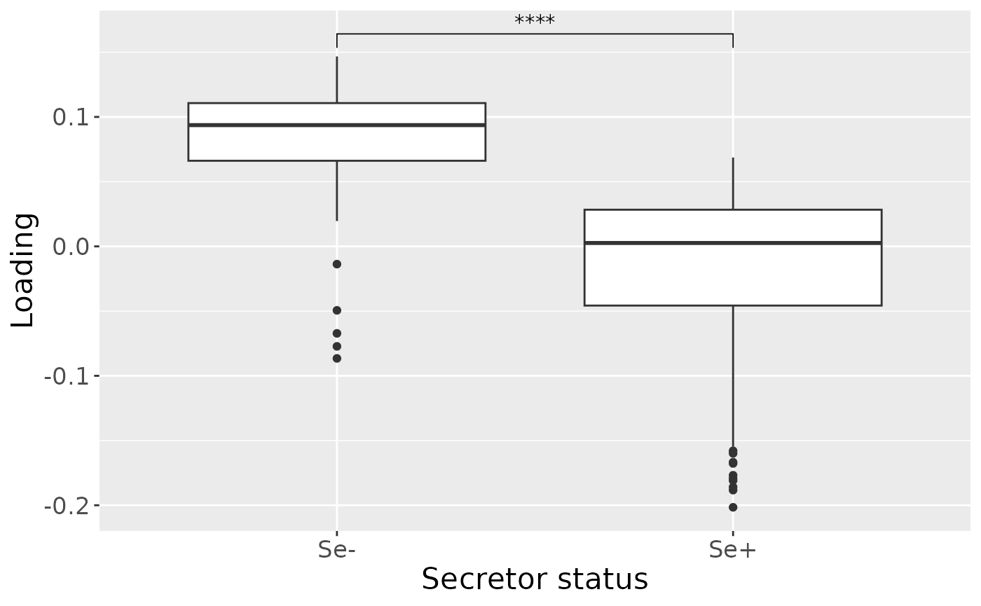
b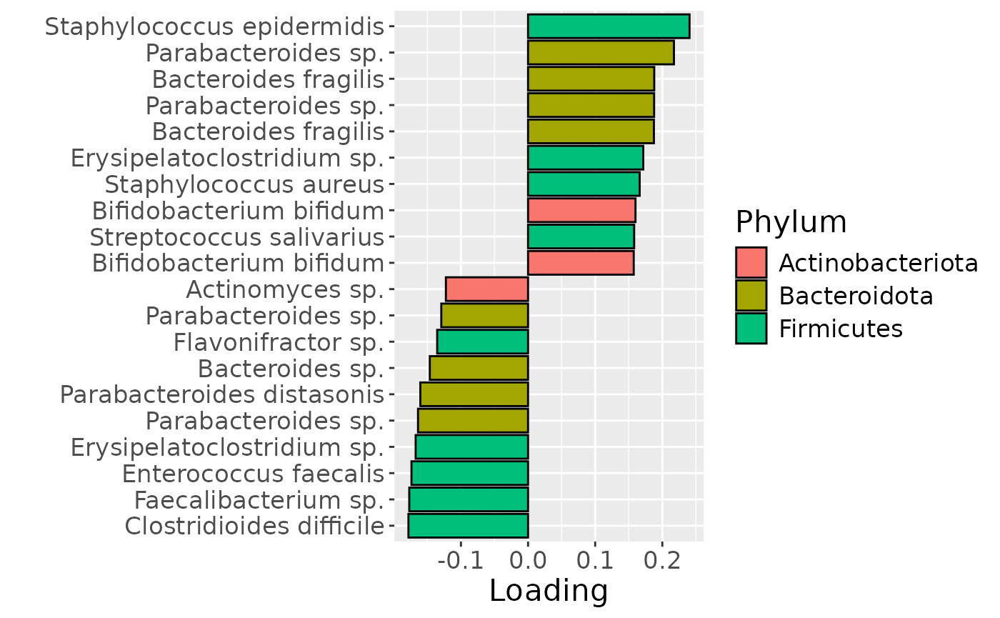
c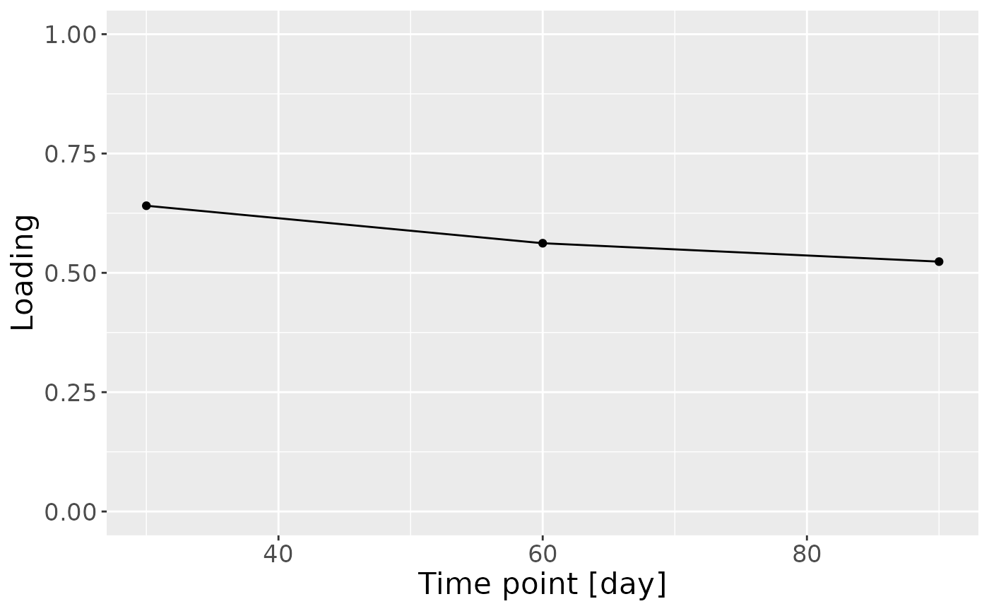
d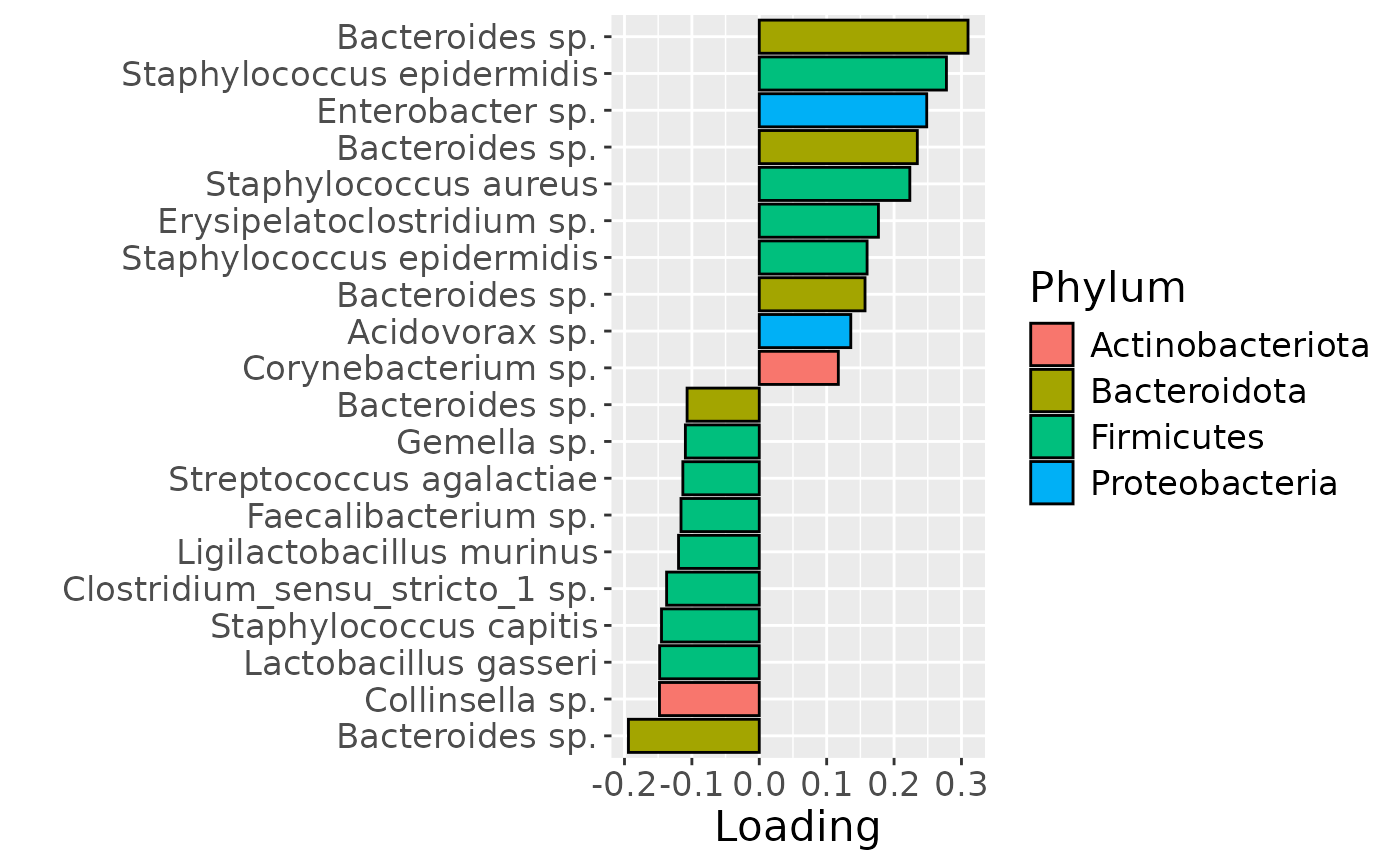
e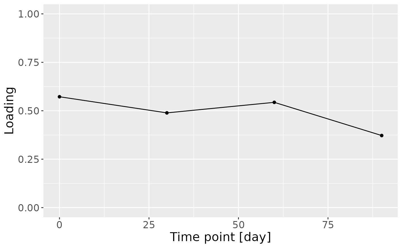
f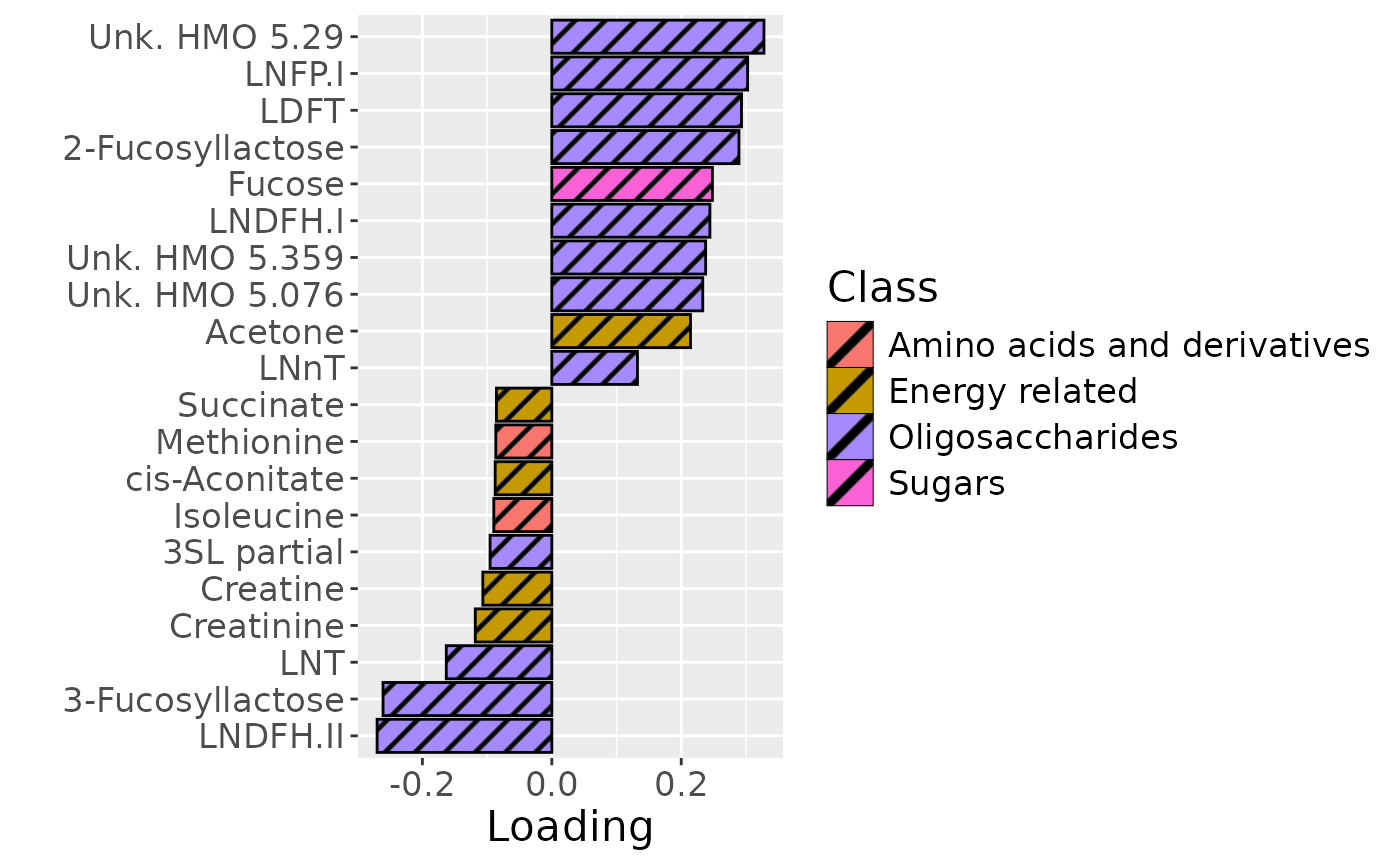
g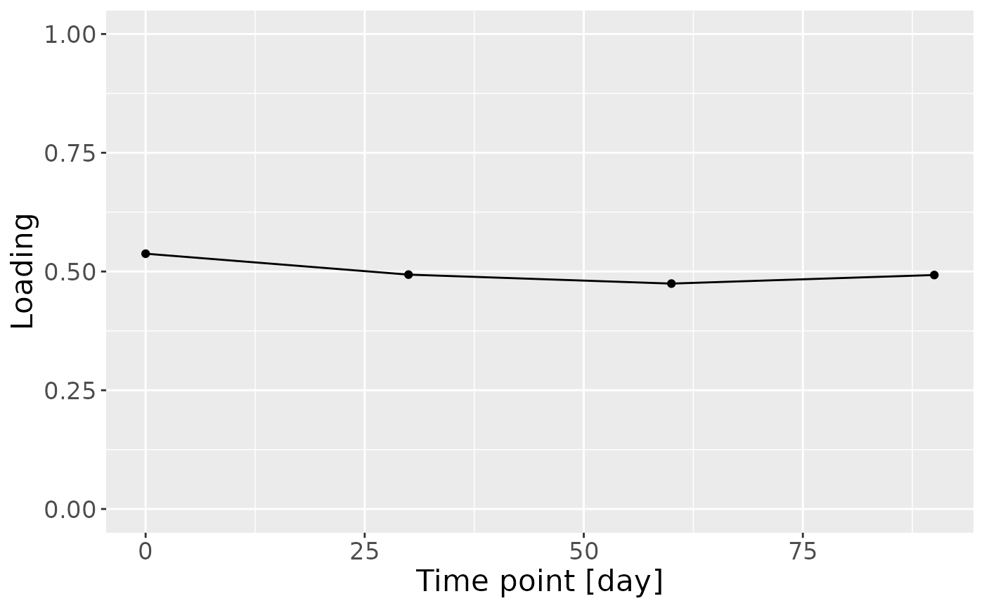
# Faeces
topIndices = processedFaeces$mode2 %>% mutate(index=1:nrow(.), Comp = model_ACMTF$Fac[[2]][,2]) %>% arrange(desc(Comp)) %>% head() %>% select(index) %>% pull()
bottomIndices = processedFaeces$mode2 %>% mutate(index=1:nrow(.), Comp = model_ACMTF$Fac[[2]][,2]) %>% arrange(desc(Comp)) %>% tail() %>% select(index) %>% pull()

Xhat = parafac4microbiome::reinflateTensor(model_ACMTF$Fac[[1]][,2], model_ACMTF$Fac[[2]][,2], model_ACMTF$Fac[[3]][,2])

print("Positive loadings:")
print(cor(Xhat[,topIndices[1],1], processedMilkMetab$mode1$Secretor))
print("Negative loadings:")
print(cor(Xhat[,bottomIndices[1],1], processedMilkMetab$mode1$Secretor))

print("Positive loadings:")
print(cor(Xhat[,topIndices[1],1], processedMilkMetab$mode1$BMI)) # flip
print("Negative loadings:")
print(cor(Xhat[,bottomIndices[1],1], processedMilkMetab$mode1$BMI))

# Milk
topIndices = processedMilk$mode2 %>% mutate(index=1:nrow(.), Comp = model_ACMTF$Fac[[4]][,2]) %>% arrange(desc(Comp)) %>% head() %>% select(index) %>% pull()
bottomIndices = processedMilk$mode2 %>% mutate(index=1:nrow(.), Comp = model_ACMTF$Fac[[4]][,2]) %>% arrange(desc(Comp)) %>% tail() %>% select(index) %>% pull()

Xhat = parafac4microbiome::reinflateTensor(model_ACMTF$Fac[[1]][,2], model_ACMTF$Fac[[4]][,2], model_ACMTF$Fac[[5]][,2])

print("Positive loadings:")
print(cor(Xhat[,topIndices[1],1], processedMilkMetab$mode1$Secretor))
print("Negative loadings:")
print(cor(Xhat[,bottomIndices[1],1], processedMilkMetab$mode1$Secretor))

print("Positive loadings:")
print(cor(Xhat[,topIndices[1],1], processedMilkMetab$mode1$BMI)) # flip
print("Negative loadings:")
print(cor(Xhat[,bottomIndices[1],1], processedMilkMetab$mode1$BMI))

# MilkMetab
topIndices = processedMilkMetab$mode2 %>% mutate(index=1:nrow(.), Comp = model_ACMTF$Fac[[6]][,2]) %>% arrange(desc(Comp)) %>% head() %>% select(index) %>% pull()
bottomIndices = processedMilkMetab$mode2 %>% mutate(index=1:nrow(.), Comp = model_ACMTF$Fac[[6]][,2]) %>% arrange(desc(Comp)) %>% tail() %>% select(index) %>% pull()

Xhat = parafac4microbiome::reinflateTensor(model_ACMTF$Fac[[1]][,2], model_ACMTF$Fac[[6]][,2], model_ACMTF$Fac[[7]][,2])

print("Positive loadings:")
print(cor(Xhat[,topIndices[1],1], processedMilkMetab$mode1$Secretor)) # NO FLIP BE CAREFUL
print("Negative loadings:")
print(cor(Xhat[,bottomIndices[1],1], processedMilkMetab$mode1$Secretor))

print("Positive loadings:")
print(cor(Xhat[,topIndices[1],1], processedMilkMetab$mode1$BMI)) # flip
print("Negative loadings:")
print(cor(Xhat[,bottomIndices[1],1], processedMilkMetab$mode1$BMI))
a = processedMilk$mode1 %>%
  mutate(Component_1 = model_ACMTF$Fac[[1]][,2]) %>%
  ggplot(aes(x=BMI,y=Component_1)) +
  geom_point() +
  stat_cor() +
  xlab("ppBMI") +
  ylab("Loading") +
  theme(text=element_text(size=16))

df = processedFaeces$mode2 %>%
  mutate(Component_1 = -1*model_ACMTF$Fac[[2]][,2]) %>%
  arrange(Component_1) %>%
  mutate(index=1:nrow(.)) %>%
  mutate(Genus = gsub("g__", "", V7), Species = gsub("s__", "", V8)) %>%
  mutate(Species = str_split_fixed(Species, "_", 2)[,2]) %>%
  mutate(dplyr::across(.cols = Species, .fns = ~ dplyr::if_else(stringr::str_detect(.x, "sp."), "", .x))) %>%
  mutate(dplyr::across(.cols = Species, .fns = ~ dplyr::if_else(stringr::str_detect(.x, "organism"), "", .x))) %>%
  mutate(dplyr::across(.cols = Species, .fns = ~ dplyr::if_else(stringr::str_detect(.x, "bacterium"), "", .x))) %>%
  filter(index %in% c(1:10, 84:93))

df[df$Genus == "" & df$Species == "", "Species"] = "Unknown"
df[df$Species == "", "Species"] = "sp."
df$name = paste0(df$Genus, " ", df$Species)

b = df %>%
  ggplot(aes(x=Component_1,y=as.factor(index),fill=as.factor(V3))) +
  geom_bar(stat="identity", col="black") +
  xlab("Loading") +
  ylab("") +
  scale_y_discrete(labels=df$name) +
  scale_fill_manual(name="Phylum", values=hue_pal()(5)[-5], labels=c("Actinobacteriota", "Bacteroidota", "Firmicutes", "Proteobacteria")) +
  theme(text=element_text(size=16))

c = model_ACMTF$Fac[[3]][,2] %>%
  as_tibble() %>%
  mutate(value=value) %>%
  ggplot(aes(x=c(30,60,90),y=value)) +
  geom_line() +
  geom_point() +
  xlab("Time point [day]") +
  ylab("Loading") +
  ylim(0,1) +
  theme(text=element_text(size=16))

df = processedMilk$mode2 %>%
  mutate(Component_1 = -1*model_ACMTF$Fac[[4]][,2]) %>%
  arrange(Component_1) %>%
  mutate(index=1:nrow(.)) %>%
  mutate(Genus = gsub("g__", "", V7), Species = gsub("s__", "", V8)) %>%
  mutate(Species = str_split_fixed(Species, "_", 2)[,2]) %>%
  mutate(dplyr::across(.cols = Species, .fns = ~ dplyr::if_else(stringr::str_detect(.x, "sp."), "", .x))) %>%
  mutate(dplyr::across(.cols = Species, .fns = ~ dplyr::if_else(stringr::str_detect(.x, "organism"), "", .x))) %>%
  mutate(dplyr::across(.cols = Species, .fns = ~ dplyr::if_else(stringr::str_detect(.x, "bacterium"), "", .x))) %>%
  filter(index %in% c(1:10, 106:115))

df[df$Genus == "" & df$Species == "", "Species"] = "Unknown"
df[df$Species == "", "Species"] = "sp."
df$name = paste0(df$Genus, " ", df$Species)

d = df %>%
  ggplot(aes(x=Component_1,y=as.factor(index),fill=as.factor(V3))) +
  geom_bar(stat="identity", col="black") +
  xlab("Loading") +
  ylab("") +
  scale_y_discrete(labels=df$name) +
  scale_fill_manual(name="Phylum", values=hue_pal()(5)[-c(2,5)], labels=c("Actinobacteriota", "Firmicutes", "Proteobacteria")) +
  theme(text=element_text(size=16))

e = model_ACMTF$Fac[[5]][,2] %>%
  as_tibble() %>%
  mutate(value=value) %>%
  ggplot(aes(x=c(0,30,60,90),y=value)) +
  geom_line() +
  geom_point() +
  xlab("Time point [day]") +
  ylab("Loading") +
  ylim(0,1) +
  theme(text=element_text(size=16))

temp = processedMilkMetab$mode2 %>%
  mutate(Component_1 = -1*model_ACMTF$Fac[[6]][,2]) %>%
  arrange(Component_1) %>%
  mutate(index=1:nrow(.)) %>%
  filter(index %in% c(1:10, 61:70))

f=temp %>%
  ggplot(aes(x=Component_1,y=as.factor(index),fill=as.factor(Class),pattern=as.factor(Class))) +
  geom_bar_pattern(stat="identity",
                   colour="black",
                   pattern="stripe",
                   pattern_fill="black",
                   pattern_density=0.2,
                   pattern_spacing=0.05,
                   pattern_angle=45,
                   pattern_size=0.2) +
  scale_y_discrete(label=temp$Metabolite) +
  xlab("Loading") +
  ylab("") +
  scale_fill_manual(name="Class", values=hue_pal()(7)[-c(3,5)], labels=c("Amino acids and derivatives", "Energy related", "Food derived", "Oligosaccharides", "Sugars")) +
  theme(text=element_text(size=16))

g = model_ACMTF$Fac[[7]][,2] %>%
  as_tibble() %>%
  mutate(value=value) %>%
  ggplot(aes(x=c(0,30,60,90),y=value)) +
  geom_line() +
  geom_point() +
  xlab("Time point [day]") +
  ylab("Loading") +
  ylim(0,1) +
  theme(text=element_text(size=16))

a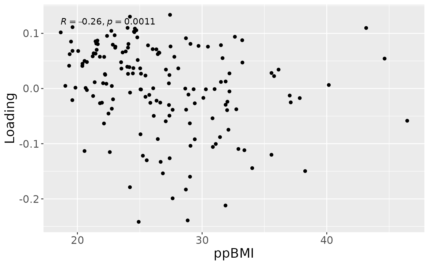
b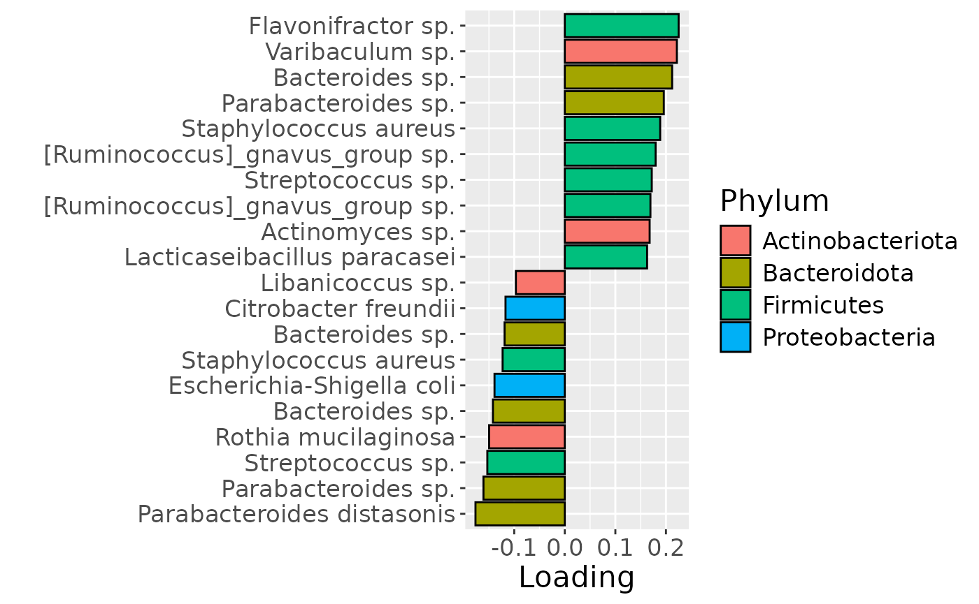
c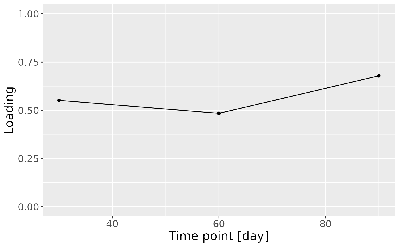
d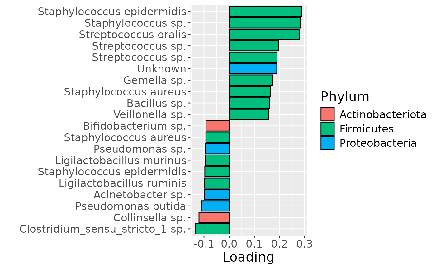
e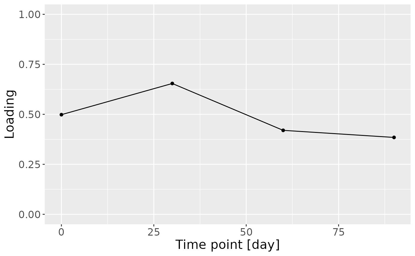
f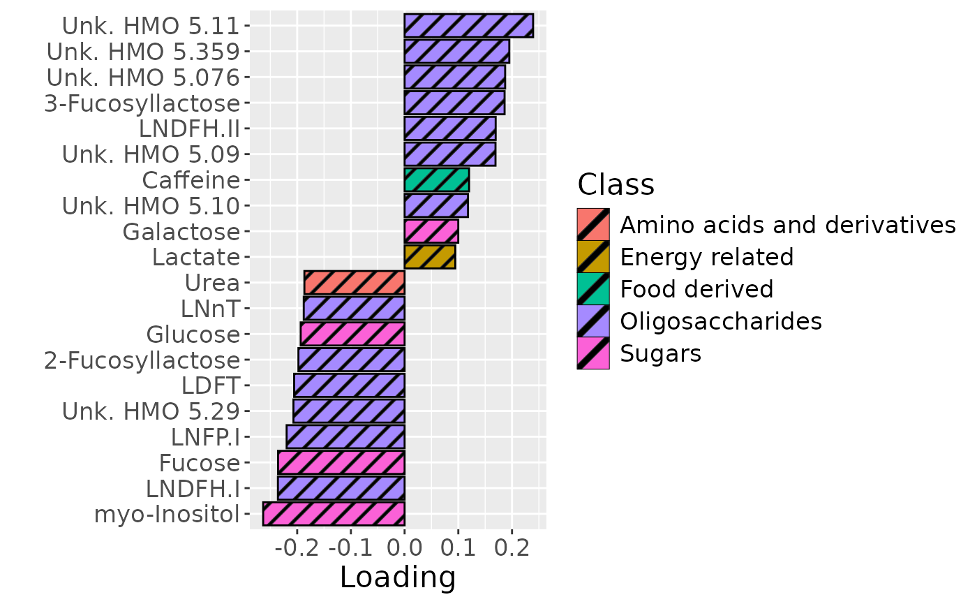
g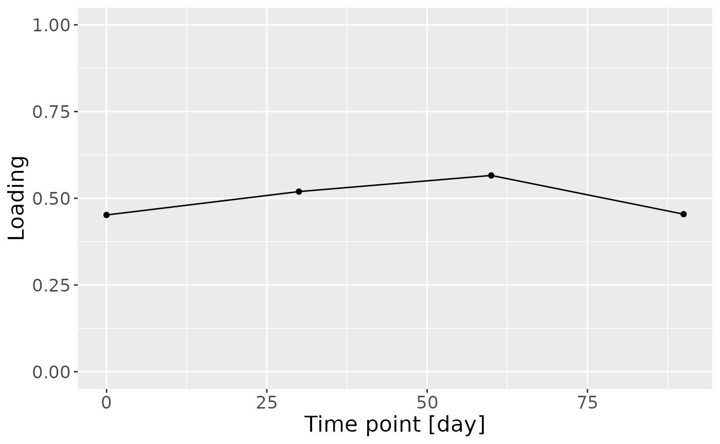
ACMTF-R
Processing
# Please see the separate R scripts at https://doi.org/10.5281/zenodo.16993009 for the model selection.
model_bmi85 = readRDS("./MAINHEALTH/ACMTFR_model_bmi85.RDS")
model_bmi85$varExp
#> [1] 5.384826 4.348941 1.778523
Description
ACMTF-R was applied to supervise the joint decomposition using maternal ppBMI as dependent variable (y). The model selection procedure revealed that one component was optimal for 0.5 <= pi <= 0.9, based on high and stable FMS CV and an RMSECV minimum. Subsequently, the one-component ACMTF-R model using pi=0.85 was selected for further interpretation due to balancing explaining the independent data and predicting y. The model explained 5.4%, 4.4%, 1.8%, and 62.1% of the variation in the infant faecal microbiome, HM microbiome, and HM metabolomics, and y, respectively.
The Lambda-matrix of the model revealed that the component was predominantly local to the infant faecal and HM microbiome data blocks, with a moderate contribution from the HM metabolomics block. However, MLR analysis revealed that the model captured variation strongly associated with maternal ppBMI and weakly associated with maternal Lewis status. This component was further inspected due to the strong association with maternal ppBMI.
testMetadata(model_bmi85, 1, processedFaeces)
#>        Term  Estimate                                        CI      P_value
#> 1       BMI -12.54749 -0.0141506288062251 – -0.0109443440288576 8.871981e-31
#> 2 C.section -18.07510  -0.0474049054595348 – 0.0112547018647361 2.248660e-01
#> 3  Secretor -12.34442 -0.0326149679423391 – 0.00792613218036735 2.303643e-01
#> 4     Lewis  59.60359   0.00222536719880014 – 0.116981813379254 4.187674e-02
#> 5    whz.6m   2.41258  -0.0052639235793006 – 0.0100890833389792 5.350509e-01
#>       P_adjust
#> 1 4.435990e-30
#> 2 2.879553e-01
#> 3 2.879553e-01
#> 4 1.046918e-01
#> 5 5.350509e-01
lambda = abs(model_bmi85$Fac[[8]])
colnames(lambda) = paste0("C", 1)

lambda %>%
  as_tibble() %>%
  mutate(block=c("Infant faecal microbiome", "HM microbiome", "HM metabolome")) %>%
  # mutate(block=factor(block, levels=c("tongue", "lowling", "lowinter", "upling", "upinter", "saliva", "metab"))) %>%
  pivot_longer(-block) %>%
  ggplot(aes(x=as.factor(name),y=value,fill=as.factor(block))) +
  geom_bar(stat="identity",position=position_dodge(),col="black") +
  xlab("ACMTF-R component number") +
  ylab(expression(lambda)) +
  scale_x_discrete(labels=1:3) +
  scale_fill_manual(name="Dataset",values = hue_pal()(3),labels=c("HM metabolome", "HM microbiome", "Infant faecal microbiome")) +
  theme(legend.position="top")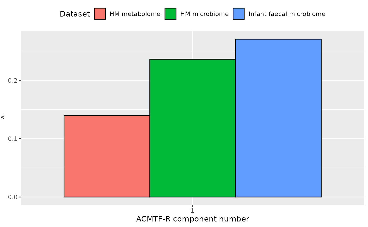
# Faeces
topIndices = processedFaeces$mode2 %>% mutate(index=1:nrow(.), Comp = model_bmi85$Fac[[2]][,1]) %>% arrange(desc(Comp)) %>% head() %>% select(index) %>% pull()
bottomIndices = processedFaeces$mode2 %>% mutate(index=1:nrow(.), Comp = model_bmi85$Fac[[2]][,1]) %>% arrange(desc(Comp)) %>% tail() %>% select(index) %>% pull()

Xhat = parafac4microbiome::reinflateTensor(model_bmi85$Fac[[1]][,1], model_bmi85$Fac[[2]][,1], model_bmi85$Fac[[3]][,1])

print("Positive loadings:")
#> [1] "Positive loadings:"
print(cor(Xhat[,topIndices[1],1], processedFaeces$mode1$BMI)) # flip
#> [1] -0.7880436
print("Negative loadings:")
#> [1] "Negative loadings:"
print(cor(Xhat[,bottomIndices[1],1], processedFaeces$mode1$BMI))
#> [1] 0.7880436

# Milk
topIndices = processedMilk$mode2 %>% mutate(index=1:nrow(.), Comp = model_bmi85$Fac[[4]][,1]) %>% arrange(desc(Comp)) %>% head() %>% select(index) %>% pull()
bottomIndices = processedMilk$mode2 %>% mutate(index=1:nrow(.), Comp = model_bmi85$Fac[[4]][,1]) %>% arrange(desc(Comp)) %>% tail() %>% select(index) %>% pull()

Xhat = parafac4microbiome::reinflateTensor(model_bmi85$Fac[[1]][,1], model_bmi85$Fac[[4]][,1], model_bmi85$Fac[[5]][,1])

print("Positive loadings:")
#> [1] "Positive loadings:"
print(cor(Xhat[,topIndices[1],1], processedFaeces$mode1$BMI)) # no flip
#> [1] 0.7880436
print("Negative loadings:")
#> [1] "Negative loadings:"
print(cor(Xhat[,bottomIndices[1],1], processedFaeces$mode1$BMI))
#> [1] -0.7880436

# Milk Metab
topIndices = processedMilkMetab$mode2 %>% mutate(index=1:nrow(.), Comp = model_bmi85$Fac[[6]][,1]) %>% arrange(desc(Comp)) %>% head() %>% select(index) %>% pull()
bottomIndices = processedMilkMetab$mode2 %>% mutate(index=1:nrow(.), Comp = model_bmi85$Fac[[6]][,1]) %>% arrange(desc(Comp)) %>% tail() %>% select(index) %>% pull()

Xhat = parafac4microbiome::reinflateTensor(model_bmi85$Fac[[1]][,1], model_bmi85$Fac[[6]][,1], model_bmi85$Fac[[7]][,1])

print("Positive loadings:")
#> [1] "Positive loadings:"
print(cor(Xhat[,topIndices[1],1], processedFaeces$mode1$BMI)) # no flip
#> [1] 0.7880436
print("Negative loadings:")
#> [1] "Negative loadings:"
print(cor(Xhat[,bottomIndices[1],1], processedFaeces$mode1$BMI))
#> [1] -0.7880436

# Faeces
df = processedFaeces$mode2 %>%
  mutate(Comp=-1*model_bmi85$Fac[[2]][,1]) %>%
  arrange(Comp) %>%
  mutate(index=1:nrow(.), name=paste0(V7," ", V8)) %>%
  mutate(Genus = gsub("g__", "", V7), Species = gsub("s__", "", V8)) %>%
  mutate(Species = str_split_fixed(Species, "_", 2)[,2]) %>%
  mutate(dplyr::across(.cols = Species, .fns = ~ dplyr::if_else(stringr::str_detect(.x, "sp."), "", .x))) %>%
  mutate(dplyr::across(.cols = Species, .fns = ~ dplyr::if_else(stringr::str_detect(.x, "organism"), "", .x))) %>%
  mutate(dplyr::across(.cols = Species, .fns = ~ dplyr::if_else(stringr::str_detect(.x, "bacterium"), "", .x))) %>%
  filter(index %in% c(1:10, 84:93))

df[df$Genus == "" & df$Species == "", "Species"] = "Unknown"
df[df$Species == "", "Species"] = "sp."
df$name = paste0(df$Genus, " ", df$Species)

a=df %>%
  ggplot(aes(x=Comp,y=as.factor(index),fill=as.factor(V3))) +
  geom_bar(stat="identity", col="black") +
  scale_y_discrete(label=df$name) +
  xlab("Loading") +
  ylab("") +
  theme(text=element_text(size=16)) +
  scale_fill_manual(name="Phylum", values=hue_pal()(5)[-5], labels=c("Actinobacteriota", "Bacteroidota", "Firmicutes", "Proteobacteria"))

# Milk
df = processedMilk$mode2 %>% mutate(Comp=model_bmi85$Fac[[4]][,1]) %>%
  arrange(Comp) %>%
  mutate(index=1:nrow(.), name=paste0(V7," ", V8)) %>%
  mutate(Genus = gsub("g__", "", V7), Species = gsub("s__", "", V8)) %>%
  mutate(Species = str_split_fixed(Species, "_", 2)[,2]) %>%
  mutate(dplyr::across(.cols = Species, .fns = ~ dplyr::if_else(stringr::str_detect(.x, "sp."), "", .x))) %>%
  mutate(dplyr::across(.cols = Species, .fns = ~ dplyr::if_else(stringr::str_detect(.x, "organism"), "", .x))) %>%
  mutate(dplyr::across(.cols = Species, .fns = ~ dplyr::if_else(stringr::str_detect(.x, "bacterium"), "", .x))) %>%
  filter(index %in% c(1:10, 106:115))

df[df$Genus == "" & df$Species == "", "Species"] = "Unknown"
df[df$Species == "", "Species"] = "sp."
df$name = paste0(df$Genus, " ", df$Species)

b=df %>%
  ggplot(aes(x=Comp,y=as.factor(index),fill=as.factor(V3))) +
  geom_bar(stat="identity", col="black") +
  scale_y_discrete(label=df$name) +
  xlab("Loading") +
  ylab("") +
  theme(text=element_text(size=16)) +
  scale_fill_manual(name="Phylum", values=hue_pal()(5)[-5], labels=c("Actinobacteriota", "Bacteroidota", "Firmicutes", "Proteobacteria"))

# MilkMetab
df = processedMilkMetab$mode2 %>% mutate(Comp=model_bmi85$Fac[[6]][,1]) %>% arrange(Comp) %>% mutate(index=1:nrow(.), name=Metabolite) %>% filter(index %in% c(1:10, 61:70))
c=df %>%
  ggplot(aes(x=Comp,y=as.factor(index),fill=as.factor(Class),pattern=as.factor(Class))) +
  geom_bar_pattern(stat="identity",
                   colour="black",
                   pattern="stripe",
                   pattern_fill="black",
                   pattern_density=0.2,
                   pattern_spacing=0.05,
                   pattern_angle=45,
                   pattern_size=0.2) +
  scale_y_discrete(label=df$name) +
  xlab("Loading") +
  ylab("") +
  scale_fill_manual(name="Class", values=hue_pal()(7)[-5], labels=c("Amino acids and derivatives", "Energy related", "Fatty acids and derivatives", "Food derived", "Oligosaccharides", "Sugars")) +
  theme(text=element_text(size=16))

a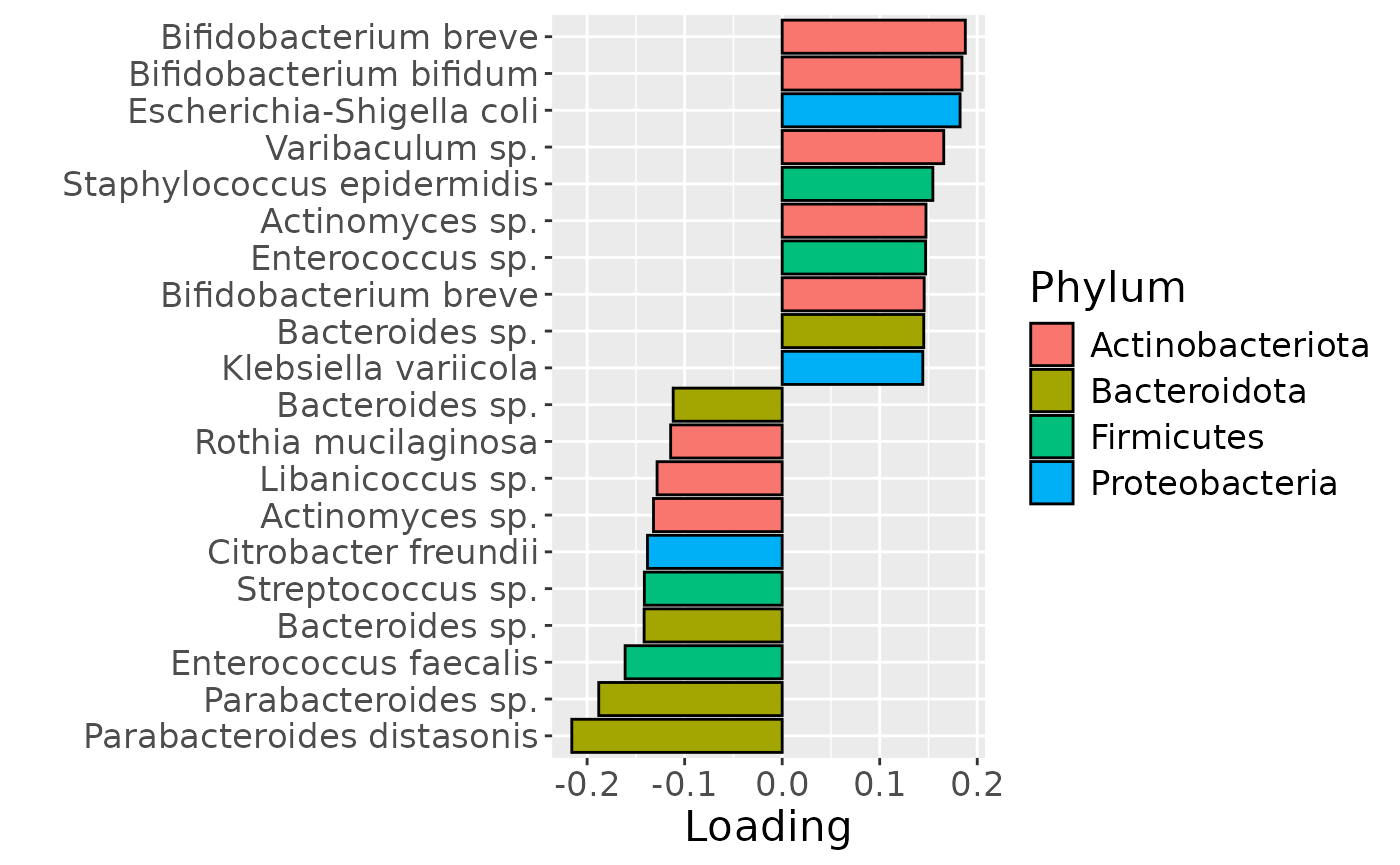
b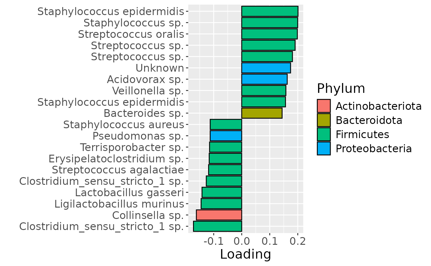
c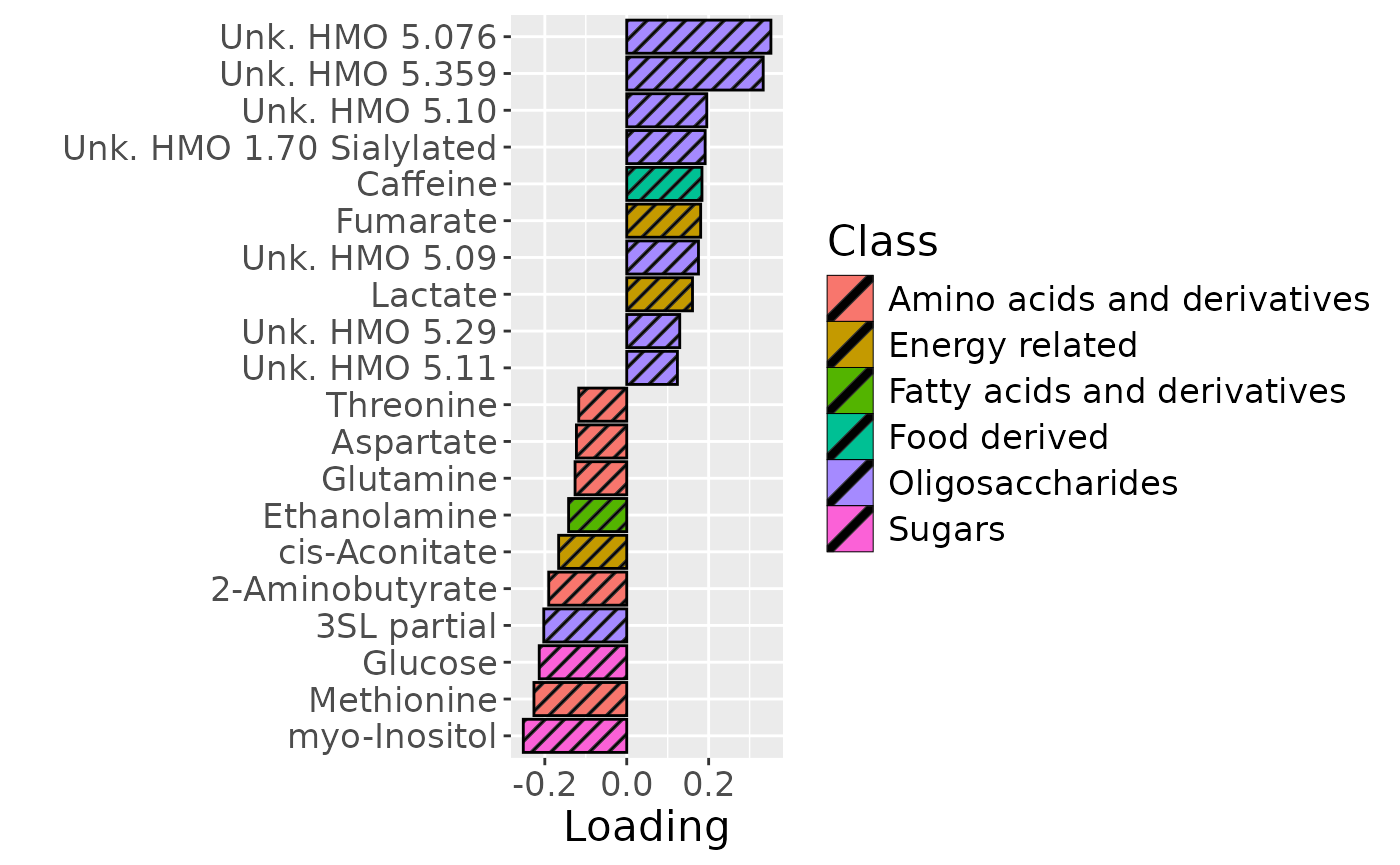
d = (model_bmi85$Fac[[3]]) %>%
  as_tibble() %>%
  mutate(time=c(30,60,90)) %>%
  pivot_longer(-time) %>%
  ggplot(aes(x=time,y=value)) +
  geom_line() +
  geom_point() +
  ylim(0,1) +
  xlab("Time point [days]") +
  ylab("Loading") +
  theme(text=element_text(size=16))
#> Warning: The `x` argument of `as_tibble.matrix()` must have unique column names if
#> `.name_repair` is omitted as of tibble 2.0.0.
#> ℹ Using compatibility `.name_repair`.
#> This warning is displayed once every 8 hours.
#> Call `lifecycle::last_lifecycle_warnings()` to see where this warning was
#> generated.

e = (-1*model_bmi85$Fac[[5]]) %>%
  as_tibble() %>%
  mutate(time=c(0,30,60,90)) %>%
  pivot_longer(-time) %>%
  ggplot(aes(x=time,y=value)) +
  geom_line() +
  geom_point() +
  ylim(0,1) +
  xlab("Time point [days]") +
  ylab("Loading") +
  theme(text=element_text(size=16))

f = (-1*model_bmi85$Fac[[7]]) %>%
  as_tibble() %>%
  mutate(time=c(0,30,60,90)) %>%
  pivot_longer(-time) %>%
  ggplot(aes(x=time,y=value)) +
  geom_line() +
  geom_point() +
  ylim(0,1) +
  xlab("Time point [days]") +
  ylab("Loading") +
  theme(text=element_text(size=16))

d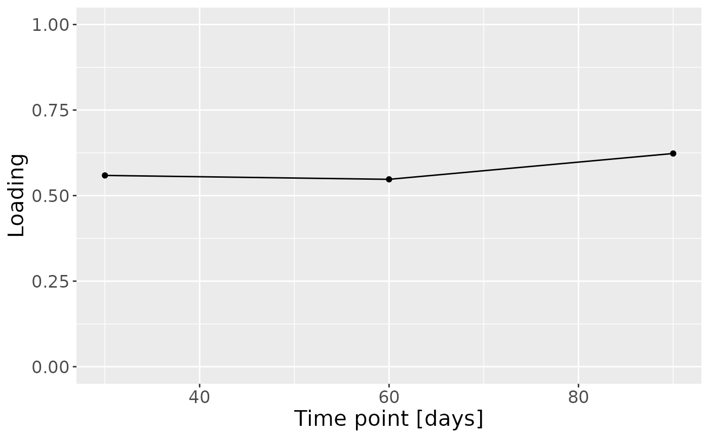
e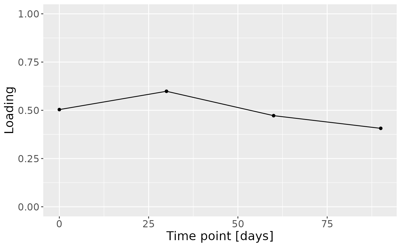
f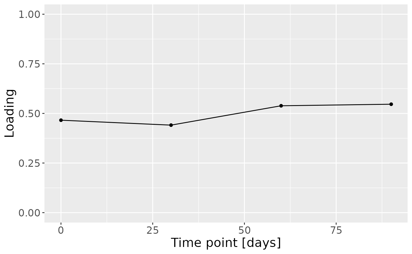
Positively loaded taxa including Bifidobacterium, Bacteroides, Enterococcus, Escherichia coli and Staphylococcus epidermidis were enriched in infants of high ppBMI mothers, and depleted in infants of low ppBMI mothers. Conversely, negatively loaded taxa including Parabacteroides, Libanicoccus and Rothia, were enriched in infants of low ppBMI mothers, and depleted in infants of high ppBMI mothers. The time mode loadings indicate that inter-subject differences due to maternal ppBMI are constant throughout the time series for this block.
In the HM microbiome, mainly Streptococcus and Staphylococcus were enriched in high ppBMI mothers and depleted in low ppBMI mothers. Conversely, Clostridium sensu stricto, Collinsella, and Lactobacillus were enriched in low ppBMI mothers and depleted in high ppBMI mothers. The time mode loadings indicate that inter-subject differences transiently increase at 30 days post-partum for this block.
In the HM metabolomics, positively loaded metabolites including lactate, caffeine, fumarate, and several unidentified HMOs had elevated levels in high ppBMI mothers and lower levels in low ppBMI mothers. Conversely, negatively loaded metabolites included several amino acids and related compounds such as 2-aminobutyrate, methionine, and cis-aconitate, had higher levels in high ppBMI mothers and lower levels in low ppBMI mothers.