TIFN2: Red fluorescent plaque development in gingivitis
2025-08-31
Source:vignettes/articles/TIFN2.Rmd
TIFN2.RmdPreamble
library(dplyr)
#>
#> Attaching package: 'dplyr'
#> The following objects are masked from 'package:stats':
#>
#>     filter, lag
#> The following objects are masked from 'package:base':
#>
#>     intersect, setdiff, setequal, union
library(tidyr)
library(parafac4microbiome)
library(NPLStoolbox)
library(CMTFtoolbox)
#>
#> Attaching package: 'CMTFtoolbox'
#> The following object is masked from 'package:NPLStoolbox':
#>
#>     npred
#> The following objects are masked from 'package:parafac4microbiome':
#>
#>     fac_to_vect, reinflateFac, reinflateTensor, vect_to_fac
library(ggplot2)
library(ggpubr)
library(scales)
library(ggpattern)
rf_data = read.csv("./TIFN2/RFdata.csv")
colnames(rf_data) = c("subject", "id", "fotonr", "day", "group", "RFgroup", "MQH", "SPS(tm)", "Area_delta_R30", "Area_delta_Rmax", "Area_delta_R30_x_Rmax", "gingiva_mean_R_over_G", "gingiva_mean_R_over_G_upper_jaw", "gingiva_mean_R_over_G_lower_jaw")
rf_data = rf_data %>% as_tibble()

rf_data[rf_data$subject == "VSTPHZ", 1] = "VSTPH2"
rf_data[rf_data$subject == "D2VZH0", 1] = "DZVZH0"
rf_data[rf_data$subject == "DLODNN", 1] = "DLODDN"
rf_data[rf_data$subject == "O3VQFX", 1] = "O3VQFQ"
rf_data[rf_data$subject == "F80LGT", 1] = "F80LGF"
rf_data[rf_data$subject == "26QQR0", 1] = "26QQrO"

rf_data2 = read.csv("./TIFN2/red_fluorescence_data.csv") %>% as_tibble()
rf_data2 = rf_data2[,c(2,4,181:192)]
rf_data = rf_data %>% left_join(rf_data2)
#> Joining with `by = join_by(id, day)`

rf = rf_data %>% select(subject, RFgroup) %>% unique()
age_gender = read.csv("./TIFN2/Ploeg_subjectMetadata.csv", sep=";")
age_gender = age_gender[2:nrow(age_gender),2:ncol(age_gender)]
age_gender = age_gender %>% as_tibble() %>% filter(onderzoeksgroep == 0) %>% select(naam, leeftijd, geslacht)
colnames(age_gender) = c("subject", "age", "gender")

# Correction for incorrect subject ids
age_gender[age_gender$subject == "VSTPHZ", 1] = "VSTPH2"
age_gender[age_gender$subject == "D2VZH0", 1] = "DZVZH0"
age_gender[age_gender$subject == "DLODNN", 1] = "DLODDN"
age_gender[age_gender$subject == "O3VQFX", 1] = "O3VQFQ"
age_gender[age_gender$subject == "F80LGT", 1] = "F80LGF"
age_gender[age_gender$subject == "26QQR0", 1] = "26QQrO"

age_gender = age_gender %>% arrange(subject)
mapping = c(-14,0,2,5,9,14,21)

testMetadata = function(model, comp, metadata){
  transformedSubjectLoadings = transformPARAFACloadings(model$Fac, 1)[,comp]
  transformedSubjectLoadings = transformedSubjectLoadings / norm(transformedSubjectLoadings, "2")

  metadata = metadata$mode1 %>% left_join(vanderPloeg2024$red_fluorescence %>% select(subject,day,Area_delta_R30,plaquepercent,bomppercent) %>% filter(day==14), by="subject")

  result = lm(transformedSubjectLoadings ~ plaquepercent + bomppercent + Area_delta_R30 + gender + age, data=metadata)

  # Extract coefficients and confidence intervals
  coef_estimates <- summary(result)$coefficients
  conf_intervals <- confint(result)

  # Remove intercept
  coef_estimates <- coef_estimates[rownames(coef_estimates) != "(Intercept)", ]
  conf_intervals <- conf_intervals[rownames(conf_intervals) != "(Intercept)", ]

  # Combine into a clean data frame
  summary_table <- data.frame(
    Term     = rownames(coef_estimates),
    Estimate = coef_estimates[, "Estimate"] * 1e3,
    CI       = paste0(
                 conf_intervals[, 1], " – ",
                 conf_intervals[, 2]
               ),
    P_value  = coef_estimates[, "Pr(>|t|)"],
    P_adjust = p.adjust(coef_estimates[, "Pr(>|t|)"], "BH"),
    row.names = NULL
  )

  return(summary_table)
}

testFeatures = function(model, metadata, componentNum, metadataVar){
  df = metadata$mode1 %>% left_join(rf_data %>% filter(day==14)) %>% left_join(age_gender)
  topIndices = metadata$mode2 %>% mutate(index=1:nrow(.), Comp = model$Fac[[2]][,componentNum]) %>% arrange(desc(Comp)) %>% head() %>% select(index) %>% pull()
  bottomIndices = metadata$mode2 %>% mutate(index=1:nrow(.), Comp = model$Fac[[2]][,componentNum]) %>% arrange(desc(Comp)) %>% tail() %>% select(index) %>% pull()

  timepoint = which(abs(model$Fac[[3]][,componentNum]) == max(abs(model$Fac[[3]][,componentNum])))

  Xhat = parafac4microbiome::reinflateTensor(model$Fac[[1]][,componentNum], model$Fac[[2]][,componentNum], model$Fac[[3]][,componentNum])
  y = df[metadataVar]

  print("Positive loadings:")
  print(cor(Xhat[,topIndices[1],timepoint], y))
  print("Negative loadings:")
  print(cor(Xhat[,bottomIndices[1],timepoint], y))
}

plotFeatures = function(mode2, model, componentNum, flip=FALSE){

  if(flip==TRUE){
    df = mode2 %>% mutate(Comp = -1*model$Fac[[2]][,componentNum]) %>% arrange(Comp) %>% filter(Species != "") %>% mutate(index=1:nrow(.), name = paste(Genus, Species))
  } else{
    df = mode2 %>% mutate(Comp = model$Fac[[2]][,componentNum]) %>% arrange(Comp) %>% filter(Species != "") %>% mutate(index=1:nrow(.), name = paste(Genus, Species))
  }
  df = rbind(df %>% head(n=10), df %>% tail(n=10))

  plot=df %>%
    ggplot(aes(x=Comp,y=as.factor(index),fill=as.factor(Phylum))) +
    geom_bar(stat="identity", col="black") +
    scale_y_discrete(label=df$name) +
    xlab("Loading") +
    ylab("") +
    guides(fill=guide_legend(title="Phylum")) +
    theme(text=element_text(size=16))

  return(plot)
}
phylum_colors = hue_pal()(7)ACMTF
Process
homogenizedSubjects = parafac4microbiome::vanderPloeg2024$metabolomics$mode1$subject
mask = parafac4microbiome::vanderPloeg2024$tongue$mode1$subject %in% homogenizedSubjects

# Tongue
temp = parafac4microbiome::vanderPloeg2024$tongue
temp$data = temp$data[mask,,]
temp$mode1 = temp$mode1[mask,]
processedTongue = processDataCube(temp, sparsityThreshold=0.50, considerGroups=TRUE, groupVariable="RFgroup", CLR=TRUE, centerMode=1, scaleMode=2)

# Lowling
temp = parafac4microbiome::vanderPloeg2024$lower_jaw_lingual
temp$data = temp$data[mask,,]
temp$mode1 = temp$mode1[mask,]
processedLowling = processDataCube(temp, sparsityThreshold=0.50, considerGroups=TRUE, groupVariable="RFgroup", CLR=TRUE, centerMode=1, scaleMode=2)

# Lowinter
temp = parafac4microbiome::vanderPloeg2024$lower_jaw_interproximal
temp$data = temp$data[mask,,]
temp$mode1 = temp$mode1[mask,]
processedLowinter = processDataCube(temp, sparsityThreshold=0.50, considerGroups=TRUE, groupVariable="RFgroup", CLR=TRUE, centerMode=1, scaleMode=2)

# Upling
temp = parafac4microbiome::vanderPloeg2024$upper_jaw_lingual
temp$data = temp$data[mask,,]
temp$mode1 = temp$mode1[mask,]
processedUpling = processDataCube(temp, sparsityThreshold=0.50, considerGroups=TRUE, groupVariable="RFgroup", CLR=TRUE, centerMode=1, scaleMode=2)

# Upinter
temp = parafac4microbiome::vanderPloeg2024$upper_jaw_interproximal
temp$data = temp$data[mask,,]
temp$mode1 = temp$mode1[mask,]
processedUpinter = processDataCube(temp, sparsityThreshold=0.50, considerGroups=TRUE, groupVariable="RFgroup", CLR=TRUE, centerMode=1, scaleMode=2)

# Saliva
temp = parafac4microbiome::vanderPloeg2024$saliva
temp$data = temp$data[mask,,]
temp$mode1 = temp$mode1[mask,]
processedSaliva = processDataCube(temp, sparsityThreshold=0.50, considerGroups=TRUE, groupVariable="RFgroup", CLR=TRUE, centerMode=1, scaleMode=2)

# Metabolomics stays the same
processedMetabolomics = parafac4microbiome::vanderPloeg2024$metabolomics

# Homogenize
datasets = list(processedTongue$data, processedLowling$data, processedLowinter$data, processedUpling$data, processedUpinter$data, processedSaliva$data, processedMetabolomics$data)
modes = list(c(1,2,3),c(1,4,5),c(1,6,7),c(1,8,9),c(1,10,11),c(1,12,13),c(1,14,15))
Z = setupCMTFdata(datasets,modes,normalize=TRUE)
Model selection
# Please see the separate R scripts at https://doi.org/10.5281/zenodo.16993009 for the model selection.
# acmtf_model = CMTFtoolbox::acmtf_opt(Z, 3, nstart = 100, method="L-BFGS", numCores=10)
acmtf_model = readRDS("./TIFN2/acmtf_model.RDS")
acmtf_model$varExp
#> [1] 26.077081 13.389771  7.070286 10.722769 12.014760 17.053897 18.279430
Description
ACMTF was applied to the capture to dominant source of variation across all data blocks. The model selection procedure revealed that FMS CV dropped below 0.9 when four components were selected. Therefore, a three-component ACMTF model was selected, explaining 26.1%, 13.4%, 7.1%, 10.7%, 12.0%, and 17.1% of the variation in the tongue, lower jaw lingual, lower jaw interproximal, upper jaw lingual, upper jaw interproximal, and salivary microbiome datasets, respectively, and 18.3% of the variation in the salivary metabolomics data.
The Lambda-matrix of the model revealed that the first component was predominantly local to the tongue, lower jaw lingual, upper jaw lingual, and salivary microbiome blocks, while the second component was predominantly local to the salivary metabolomics and tongue microbiome blocks, and the third component was predominantly distinct to the salivary metabolomics block. However, all components received minor contributions from other blocks as well. MLR analysis revealed that the first component captured uninterpretable variation, the second component captured variation associated with a mixture of plaque% and subject age, while the third component captured variation exclusively associated with subject age.
testMetadata(acmtf_model, 1, processedTongue)
#>             Term   Estimate                                          CI
#> 1  plaquepercent  0.4863409  -0.00506844885613745 – 0.00604113058720496
#> 2    bomppercent  2.9652292 -0.000432781614955507 – 0.00636323992350004
#> 3 Area_delta_R30  7.5900807   0.000734950049744098 – 0.0144452114121996
#> 4         gender 86.0214570      -0.010641596321994 – 0.182684510263669
#> 5            age  9.1712962   0.000577075926033553 – 0.0177655165286259
#>      P_value   P_adjust
#> 1 0.85983387 0.85983387
#> 2 0.08511896 0.10639870
#> 3 0.03102313 0.09298174
#> 4 0.07937792 0.10639870
#> 5 0.03719270 0.09298174
testMetadata(acmtf_model, 2, processedTongue)
#>             Term    Estimate                                          CI
#> 1  plaquepercent  -5.5322600 -0.0106693400579514 – -0.000395179879130161
#> 2    bomppercent   0.1529061  -0.00298958068906224 – 0.00329539294300932
#> 3 Area_delta_R30  -2.2288690  -0.00856850683903234 – 0.00411076892021208
#> 4         gender -22.1883942     -0.111582569602603 – 0.0672057811120825
#> 5            age  18.7122978     0.0107643465442291 – 0.0266602490737363
#>        P_value     P_adjust
#> 1 3.559350e-02 0.0889837601
#> 2 9.218108e-01 0.9218108424
#> 3 4.798015e-01 0.7715244490
#> 4 6.172196e-01 0.7715244490
#> 5 3.261655e-05 0.0001630827
testMetadata(acmtf_model, 3, processedTongue)
#>             Term   Estimate                                         CI
#> 1  plaquepercent  0.1361253 -0.00536264865494706 – 0.00563489919269931
#> 2    bomppercent  1.4787774  -0.0018849670226254 – 0.00484252184623444
#> 3 Area_delta_R30  4.9612353  -0.00182476661145919 – 0.0117472372709829
#> 4         gender  2.2390025    -0.0934492779583765 – 0.097927282983282
#> 5            age 14.9701758   0.00646262160971828 – 0.0234777299599013
#>       P_value    P_adjust
#> 1 0.960170260 0.962351254
#> 2 0.377912728 0.629854546
#> 3 0.146554101 0.366385252
#> 4 0.962351254 0.962351254
#> 5 0.001070941 0.005354707
lambda = abs(acmtf_model$Fac[[16]])
colnames(lambda) = paste0("C", 1:3)

lambda %>%
  as_tibble() %>%
  mutate(block=c("tongue", "lowling", "lowinter", "upling", "upinter", "saliva", "metab")) %>%
  mutate(block=factor(block, levels=c("tongue", "lowling", "lowinter", "upling", "upinter", "saliva", "metab"))) %>%
  pivot_longer(-block) %>%
  ggplot(aes(x=as.factor(name),y=value,fill=as.factor(block))) +
  geom_bar(stat="identity",position=position_dodge(),col="black") +
  xlab("ACMTF component number") +
  ylab(expression(lambda)) +
  scale_x_discrete(labels=1:3) +
  scale_fill_manual(name="Dataset",values = hue_pal()(7),labels=c("Tongue", "Lower jaw, lingual", "Lower jaw, interproximal", "Upper jaw, lingual", "Upper jaw, interproximal", "Salivary microbiome", "Salivary metabolome")) +
  theme(legend.position="top")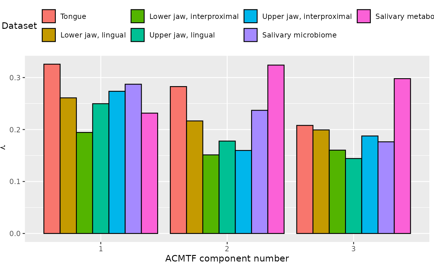
# Component 2 is interpretable as being related to age
# it is mainly described by tongue + metab

temp = list()
temp$Fac = acmtf_model$Fac[c(1,2,3)]
testFeatures(temp, processedTongue, 2, "age")
#> Joining with `by = join_by(subject, RFgroup)`
#> Joining with `by = join_by(subject, age, gender)`
#> [1] "Positive loadings:"
#>            age
#> [1,] 0.4471952
#> [1] "Negative loadings:"
#>             age
#> [1,] -0.4471952
a = plotFeatures(processedTongue$mode2, temp, 2, flip=FALSE) + scale_fill_manual(values=phylum_colors[-c(5,6,7)])

temp = list()
temp$Fac = acmtf_model$Fac[c(1,4,5)]
testFeatures(temp, processedLowling, 2, "age")
#> Joining with `by = join_by(subject, RFgroup)`
#> Joining with `by = join_by(subject, age, gender)`
#> [1] "Positive loadings:"
#>            age
#> [1,] 0.4471952
#> [1] "Negative loadings:"
#>             age
#> [1,] -0.4471952
b = plotFeatures(processedLowling$mode2, temp, 2, flip=FALSE) + scale_fill_manual(values=phylum_colors[-7])

temp = list()
temp$Fac = acmtf_model$Fac[c(1,6,7)]
testFeatures(temp, processedLowinter, 2, "age")
#> Joining with `by = join_by(subject, RFgroup)`
#> Joining with `by = join_by(subject, age, gender)`
#> [1] "Positive loadings:"
#>            age
#> [1,] 0.4471952
#> [1] "Negative loadings:"
#>             age
#> [1,] -0.4471952
c = plotFeatures(processedLowinter$mode2, temp, 2, flip=FALSE)

temp = list()
temp$Fac = acmtf_model$Fac[c(1,8,9)]
testFeatures(temp, processedUpling, 2, "age")
#> Joining with `by = join_by(subject, RFgroup)`
#> Joining with `by = join_by(subject, age, gender)`
#> [1] "Positive loadings:"
#>            age
#> [1,] 0.4471952
#> [1] "Negative loadings:"
#>             age
#> [1,] -0.4471952
d = plotFeatures(processedUpling$mode2, temp, 2, flip=FALSE)

temp = list()
temp$Fac = acmtf_model$Fac[c(1,10,11)]
testFeatures(temp, processedUpinter, 2, "age")
#> Joining with `by = join_by(subject, RFgroup)`
#> Joining with `by = join_by(subject, age, gender)`
#> [1] "Positive loadings:"
#>            age
#> [1,] 0.4471952
#> [1] "Negative loadings:"
#>             age
#> [1,] -0.4471952
e = plotFeatures(processedUpinter$mode2, temp, 2, flip=FALSE)

temp = list()
temp$Fac = acmtf_model$Fac[c(1,12,13)]
testFeatures(temp, processedSaliva, 2, "age") # flip
#> Joining with `by = join_by(subject, RFgroup)`
#> Joining with `by = join_by(subject, age, gender)`
#> [1] "Positive loadings:"
#>             age
#> [1,] -0.4471952
#> [1] "Negative loadings:"
#>            age
#> [1,] 0.4471952
f = plotFeatures(processedSaliva$mode2, temp, 2, flip=TRUE) + scale_fill_manual(values=phylum_colors[-c(3,7)])

temp = list()
temp$Fac = acmtf_model$Fac[c(1,14,15)]
testFeatures(temp, processedMetabolomics, 2, "age")
#> Joining with `by = join_by(subject, RFgroup)`
#> Joining with `by = join_by(subject, age, gender)`
#> [1] "Positive loadings:"
#>            age
#> [1,] 0.4471952
#> [1] "Negative loadings:"
#>             age
#> [1,] -0.4471952

# Metab
df = processedMetabolomics$mode2 %>% mutate(Component_2 = acmtf_model$Fac[[14]][,2]) %>% arrange(Component_2) %>% mutate(index=1:nrow(.))
df = rbind(df %>% head(n=10), df %>% tail(n=10))

g=df %>%
  ggplot(aes(x=Component_2,y=as.factor(index),fill=as.factor(Type))) +
  geom_bar(stat="identity", col="black") +
  scale_y_discrete(label=df$Name) +
  xlab("Loading") +
  ylab("") +
  guides(fill=guide_legend(title="Class")) +
  theme(text=element_text(size=16), legend.position="none")

g2 = df %>%
  ggplot(aes(x = Component_2, y = as.factor(index),
             fill = as.factor(Type),
             pattern = as.factor(Type))) +
  geom_bar_pattern(stat = "identity",
                   colour = "black",
                   pattern = "stripe",
                   pattern_fill = "black",
                   pattern_density = 0.2,
                   pattern_spacing = 0.05,
                   pattern_angle = 45,
                   pattern_size = 0.2) +
  scale_y_discrete(labels = df$Name) +
  xlab("Loading") +
  ylab("") +
  guides(fill = guide_legend(title = "Class"),
         pattern = "none") +
  theme(text = element_text(size = 16),
        legend.position = "top")

a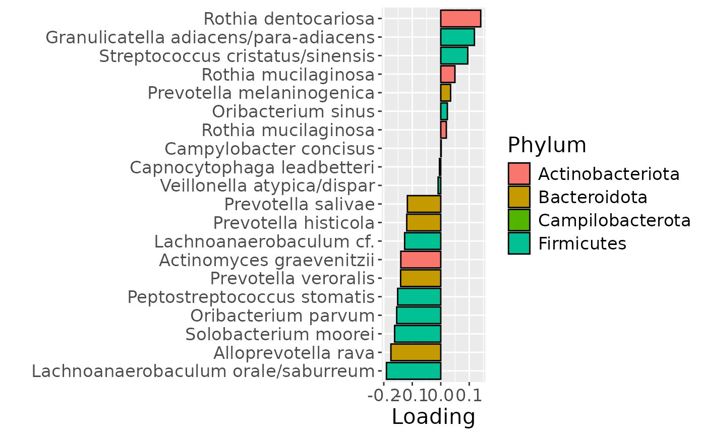
b
c
d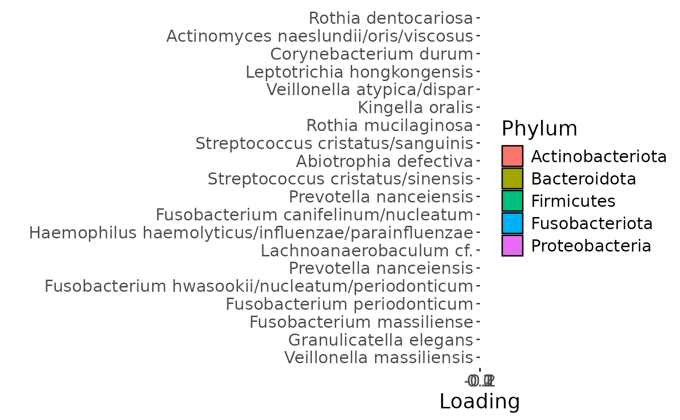
e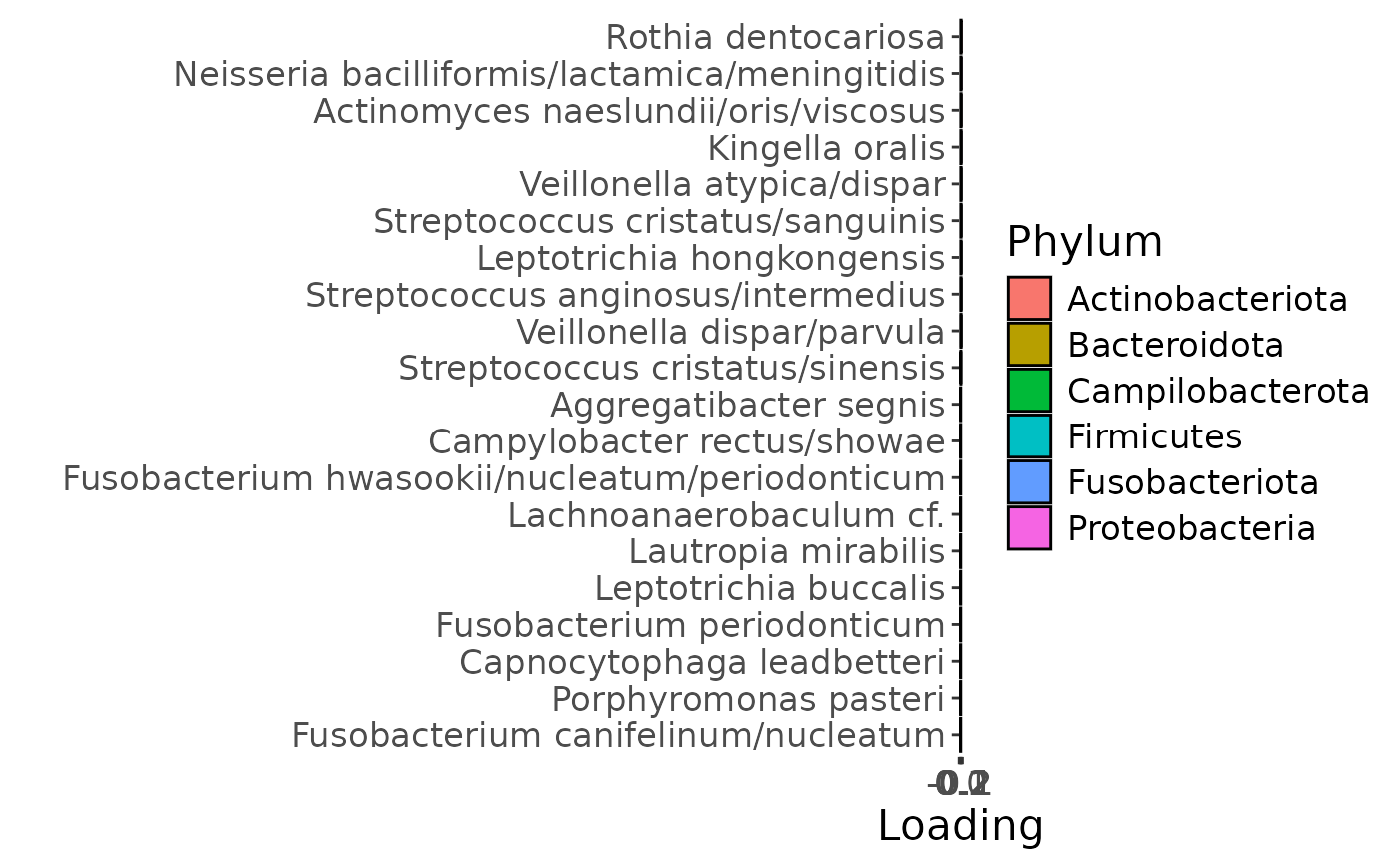
f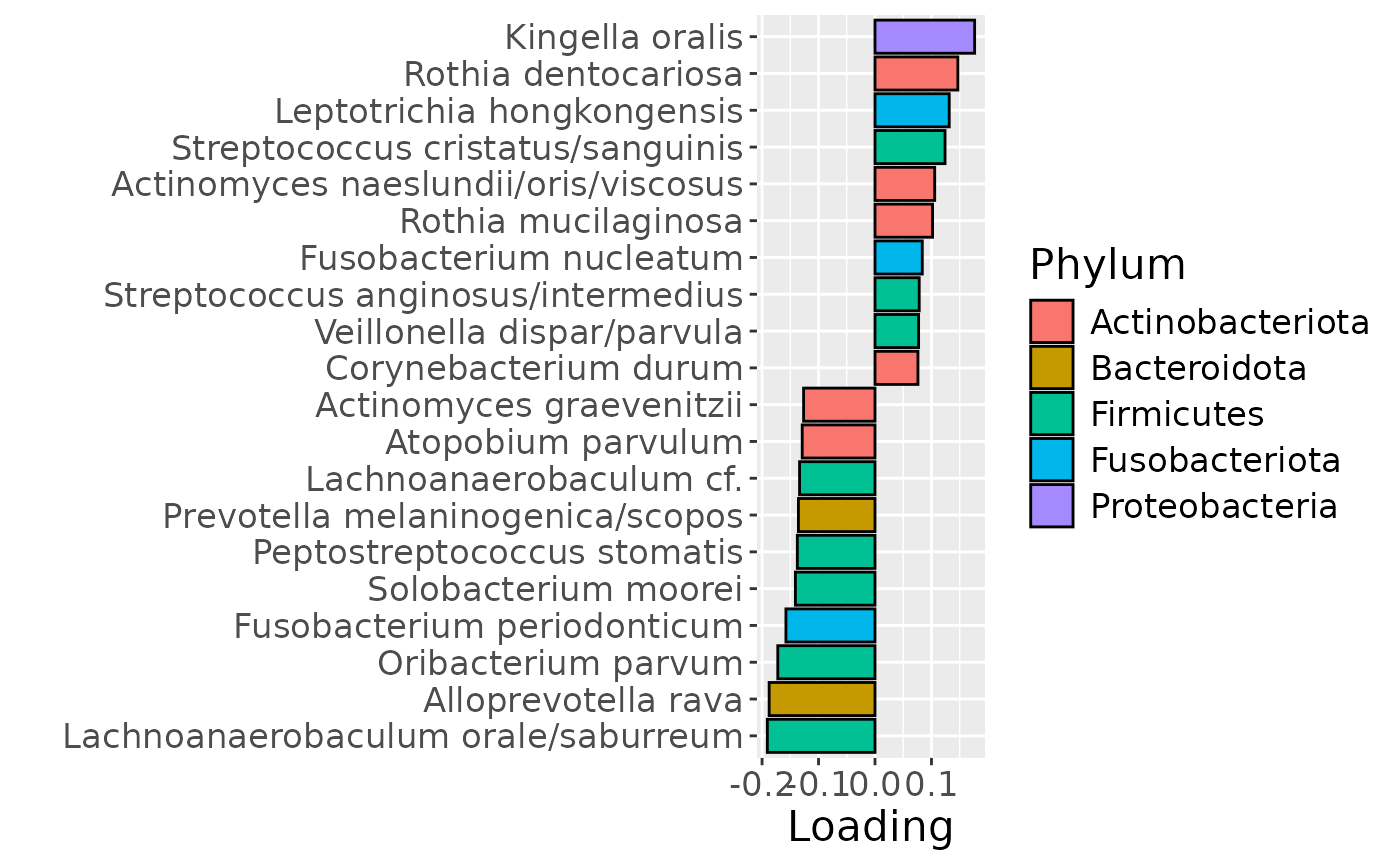
g2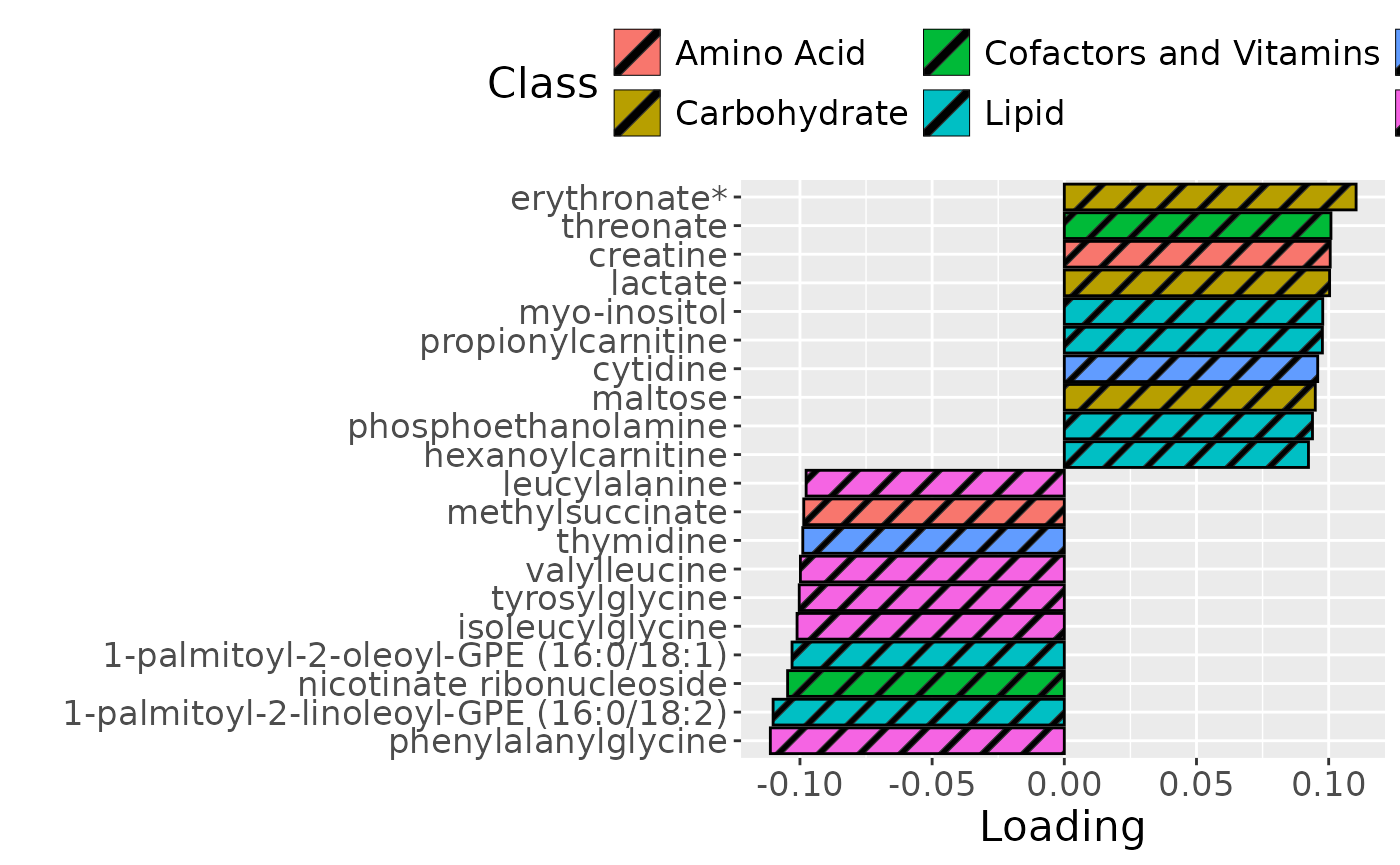
a = processedTongue$mode3 %>%
  mutate(Comp = acmtf_model$Fac[[3]][,2], day=c(-14,0,2,5,9,14,21)) %>%
  select(-visit,-status) %>%
  pivot_longer(-day) %>%
  ggplot(aes(x=day,y=value)) +
  annotate(geom = "rect", xmin = 0, xmax = 14, ymin = -Inf, ymax = Inf, fill = "red", colour = "black", alpha=0.25) +
  geom_line() +
  geom_point() +
  theme(legend.position="none") +
  xlab("Time point [days]") +
  ylab("Loading") +
  ylim(0,1)


b = processedLowling$mode3 %>%
  mutate(Comp = acmtf_model$Fac[[5]][,2], day=c(-14,0,2,5,9,14,21)) %>%
  select(-visit,-status) %>%
  pivot_longer(-day) %>%
  ggplot(aes(x=day,y=value)) +
  annotate(geom = "rect", xmin = 0, xmax = 14, ymin = -Inf, ymax = Inf, fill = "red", colour = "black", alpha=0.25) +
  geom_line() +
  geom_point() +
  theme(legend.position="none") +
  xlab("Time point [days]") +
  ylab("Loading") +
  ylim(0,1)


c = processedLowinter$mode3 %>%
  mutate(Component_1 = acmtf_model$Fac[[7]][,2], day=c(-14,0,2,5,9,14,21)) %>%
  select(-visit,-status) %>%
  pivot_longer(-day) %>%
  ggplot(aes(x=day,y=value)) +
  annotate(geom = "rect", xmin = 0, xmax = 14, ymin = -Inf, ymax = Inf, fill = "red", colour = "black", alpha=0.25) +
  geom_line() +
  geom_point() +
  theme(legend.position="none") +
  xlab("Time point [days]") +
  ylab("Loading") +
  ylim(0,1)

d = processedUpling$mode3 %>%
  mutate(Component_1 = acmtf_model$Fac[[9]][,2], day=c(-14,0,2,5,9,14,21)) %>%
  ggplot(aes(x=day,y=Component_1)) +
  annotate(geom = "rect", xmin = 0, xmax = 14, ymin = -Inf, ymax = Inf, fill = "red", colour = "black", alpha=0.25) +
  geom_line() +
  geom_point() +
  theme(legend.position="none") +
  xlab("Time point [days]") +
  ylab("Loading") +
  ylim(0,1)

e = processedUpinter$mode3 %>%
  mutate(Component_1 = acmtf_model$Fac[[11]][,2], day=c(-14,0,2,5,9,14,21)) %>%
  ggplot(aes(x=day,y=Component_1)) +
  annotate(geom = "rect", xmin = 0, xmax = 14, ymin = -Inf, ymax = Inf, fill = "red", colour = "black", alpha=0.25) +
  geom_line() +
  geom_point() +
  theme(legend.position="none") +
  xlab("Time point [days]") +
  ylab("Loading") +
  ylim(0,1)

f = processedSaliva$mode3 %>%
  mutate(Component_1 = -1*acmtf_model$Fac[[13]][,2], day=c(-14,0,2,5,9,14,21)) %>%
  ggplot(aes(x=day,y=Component_1)) +
  annotate(geom = "rect", xmin = 0, xmax = 14, ymin = -Inf, ymax = Inf, fill = "red", colour = "black", alpha=0.25) +
  geom_line() +
  geom_point() +
  theme(legend.position="none") +
  xlab("Time point [days]") +
  ylab("Loading") +
  ylim(0,1)

g = processedMetabolomics$mode3 %>%
  mutate(Component_1 = acmtf_model$Fac[[15]][,2], day=c(0,2,5,9,14)) %>%
  ggplot(aes(x=day,y=Component_1)) +
  annotate(geom = "rect", xmin = 0, xmax = 14, ymin = -Inf, ymax = Inf, fill = "red", colour = "black", alpha=0.25) +
  geom_line() +
  geom_point() +
  theme(legend.position="none") +
  xlab("Time point [days]") +
  ylab("Loading") +
  ylim(0,1)

a
b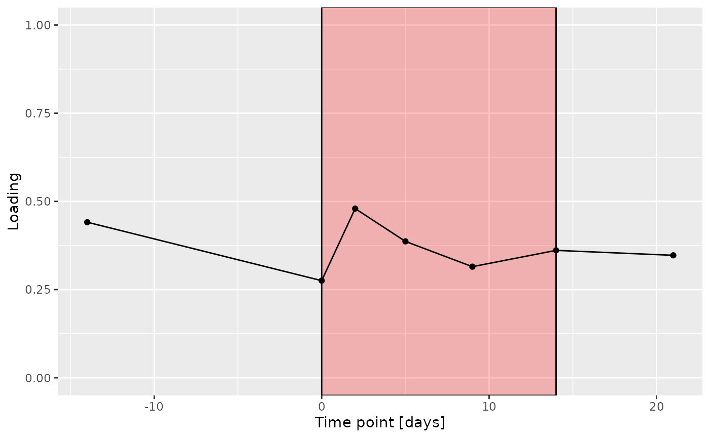
c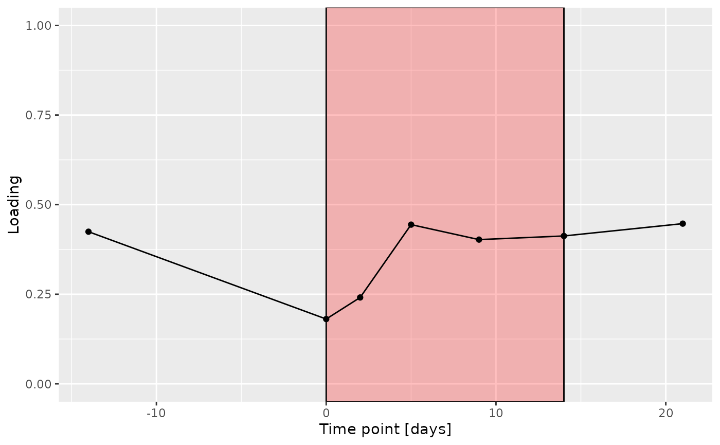
d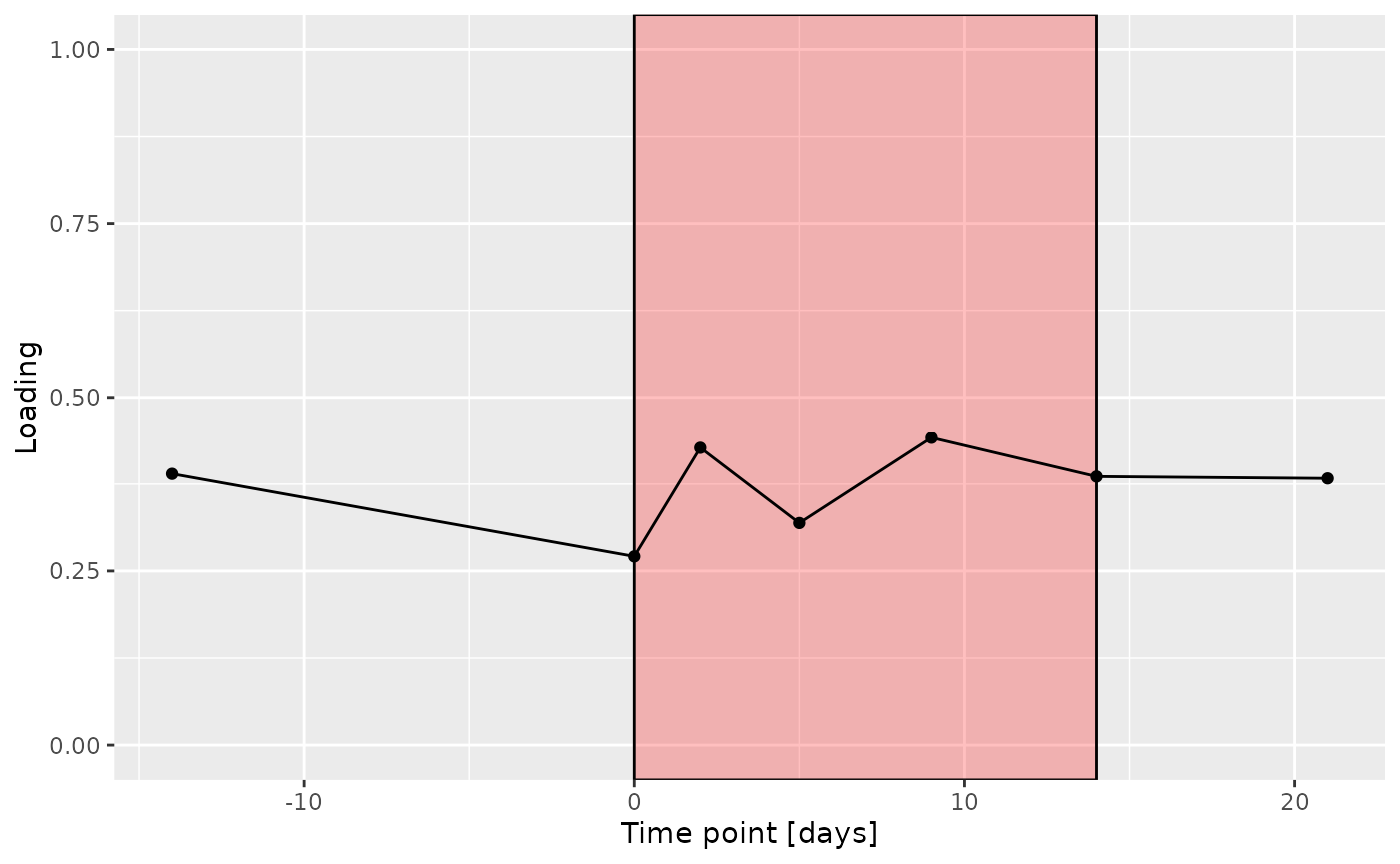
e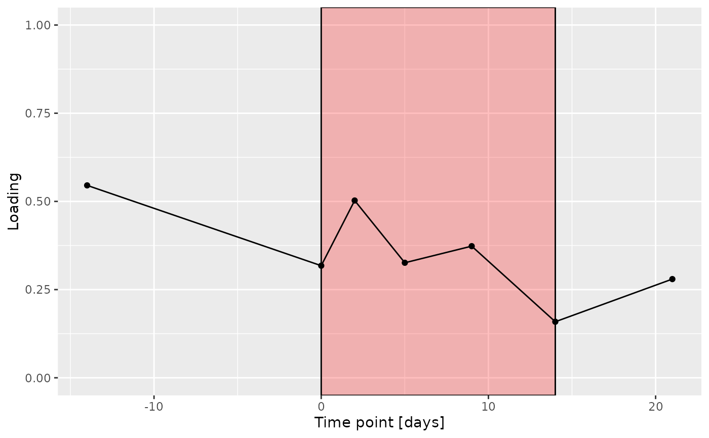
f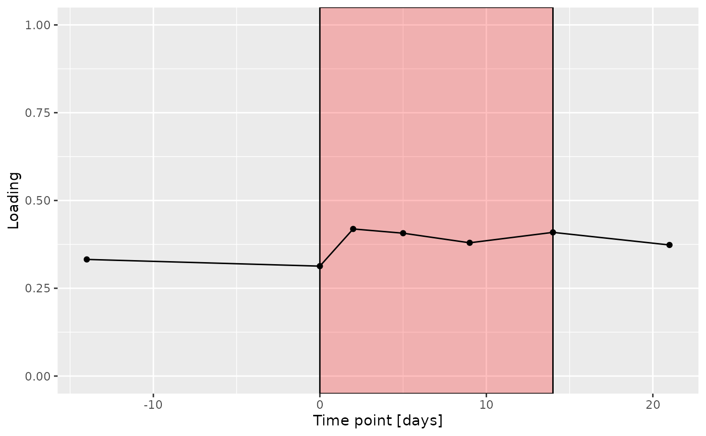
g
# Component 2 is interpretable as being related to age
# it is mainly described by tongue + metab

temp = list()
temp$Fac = acmtf_model$Fac[c(1,2,3)]
testFeatures(temp, processedTongue, 3, "age")
#> Joining with `by = join_by(subject, RFgroup)`
#> Joining with `by = join_by(subject, age, gender)`
#> [1] "Positive loadings:"
#>           age
#> [1,] 0.545521
#> [1] "Negative loadings:"
#>            age
#> [1,] -0.545521
a = plotFeatures(processedTongue$mode2, temp, 3, flip=FALSE) + scale_fill_manual(values=phylum_colors[-c(3,5,6,7)])

temp = list()
temp$Fac = acmtf_model$Fac[c(1,4,5)]
testFeatures(temp, processedLowling, 3, "age")
#> Joining with `by = join_by(subject, RFgroup)`
#> Joining with `by = join_by(subject, age, gender)`
#> [1] "Positive loadings:"
#>           age
#> [1,] 0.545521
#> [1] "Negative loadings:"
#>            age
#> [1,] -0.545521
b = plotFeatures(processedLowling$mode2, temp, 3, flip=FALSE) + scale_fill_manual(values=phylum_colors[-c(3,7)])

temp = list()
temp$Fac = acmtf_model$Fac[c(1,6,7)]
testFeatures(temp, processedLowinter, 3, "age") # flip
#> Joining with `by = join_by(subject, RFgroup)`
#> Joining with `by = join_by(subject, age, gender)`
#> [1] "Positive loadings:"
#>            age
#> [1,] -0.545521
#> [1] "Negative loadings:"
#>           age
#> [1,] 0.545521
c = plotFeatures(processedLowinter$mode2, temp, 3, flip=TRUE) + scale_fill_manual(values=phylum_colors[-c(3,7)])

temp = list()
temp$Fac = acmtf_model$Fac[c(1,8,9)]
testFeatures(temp, processedUpling, 3, "age") # cor says flip, but lambda is negative -> no flip
#> Joining with `by = join_by(subject, RFgroup)`
#> Joining with `by = join_by(subject, age, gender)`
#> [1] "Positive loadings:"
#>            age
#> [1,] -0.545521
#> [1] "Negative loadings:"
#>           age
#> [1,] 0.545521
d = plotFeatures(processedUpling$mode2, temp, 3, flip=FALSE) + scale_fill_manual(values=phylum_colors[-c(3,7)])

temp = list()
temp$Fac = acmtf_model$Fac[c(1,10,11)]
testFeatures(temp, processedUpinter, 3, "age")
#> Joining with `by = join_by(subject, RFgroup)`
#> Joining with `by = join_by(subject, age, gender)`
#> [1] "Positive loadings:"
#>           age
#> [1,] 0.545521
#> [1] "Negative loadings:"
#>            age
#> [1,] -0.545521
e = plotFeatures(processedUpinter$mode2, temp, 3, flip=FALSE) + scale_fill_manual(values=phylum_colors[-c(3,7)])

temp = list()
temp$Fac = acmtf_model$Fac[c(1,12,13)]
testFeatures(temp, processedSaliva, 3, "age") # flip
#> Joining with `by = join_by(subject, RFgroup)`
#> Joining with `by = join_by(subject, age, gender)`
#> [1] "Positive loadings:"
#>            age
#> [1,] -0.545521
#> [1] "Negative loadings:"
#>            age
#> [1,] -0.545521
f = plotFeatures(processedSaliva$mode2, temp, 3, flip=TRUE) + scale_fill_manual(values=phylum_colors[-c(3,7)])

temp = list()
temp$Fac = acmtf_model$Fac[c(1,14,15)]
testFeatures(temp, processedMetabolomics, 3, "age") # flip
#> Joining with `by = join_by(subject, RFgroup)`
#> Joining with `by = join_by(subject, age, gender)`
#> [1] "Positive loadings:"
#>            age
#> [1,] -0.545521
#> [1] "Negative loadings:"
#>           age
#> [1,] 0.545521

# Metab
df = processedMetabolomics$mode2 %>% mutate(Component_2 = -1*acmtf_model$Fac[[14]][,3]) %>% arrange(Component_2) %>% mutate(index=1:nrow(.))
df = rbind(df %>% head(n=10), df %>% tail(n=10))

g=df %>%
  ggplot(aes(x=Component_2,y=as.factor(index),fill=as.factor(Type))) +
  geom_bar(stat="identity", col="black") +
  scale_y_discrete(label=df$Name) +
  xlab("Loading") +
  ylab("") +
  guides(fill=guide_legend(title="Class")) +
  theme(text=element_text(size=16), legend.position="none")

g2 = df %>%
  ggplot(aes(x = Component_2, y = as.factor(index),
             fill = as.factor(Type),
             pattern = as.factor(Type))) +
  geom_bar_pattern(stat = "identity",
                   colour = "black",
                   pattern = "stripe",
                   pattern_fill = "black",
                   pattern_density = 0.2,
                   pattern_spacing = 0.05,
                   pattern_angle = 45,
                   pattern_size = 0.2) +
  scale_y_discrete(labels = df$Name) +
  xlab("Loading") +
  ylab("") +
  guides(fill = guide_legend(title = "Class"),
         pattern = "none") +
  theme(text = element_text(size = 16),
        legend.position = "top")

a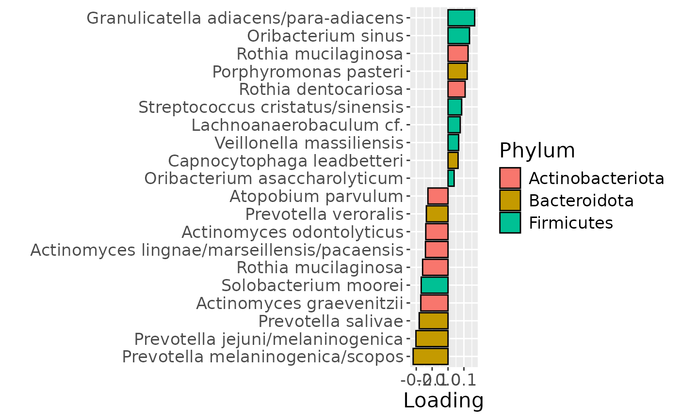
b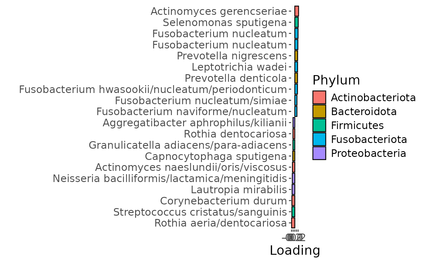
c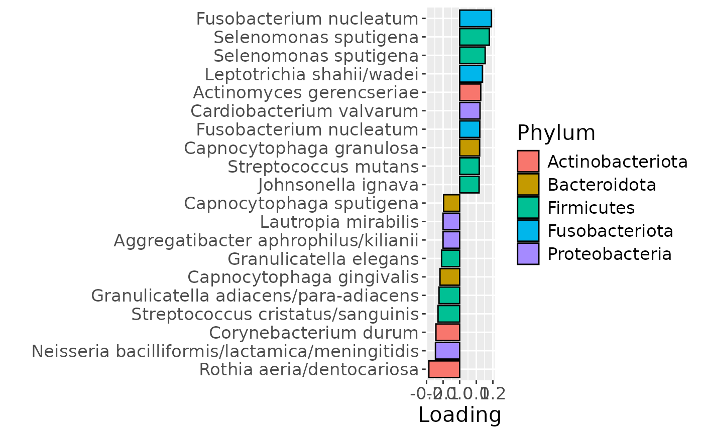
d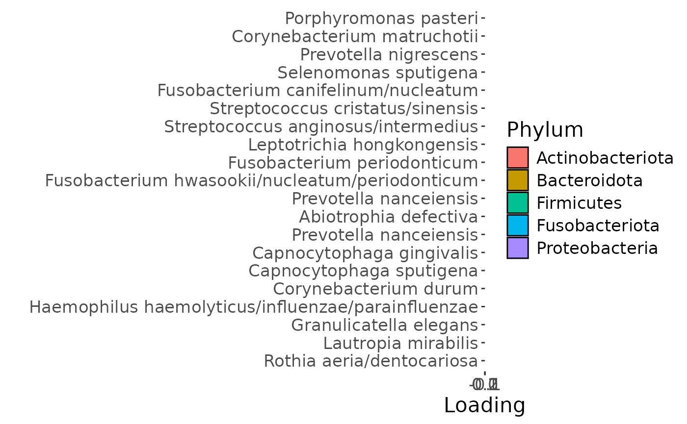
e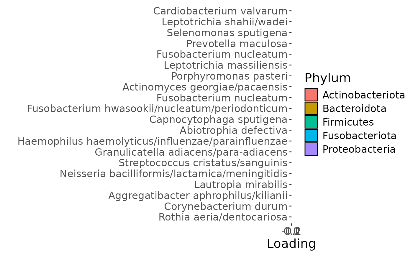
f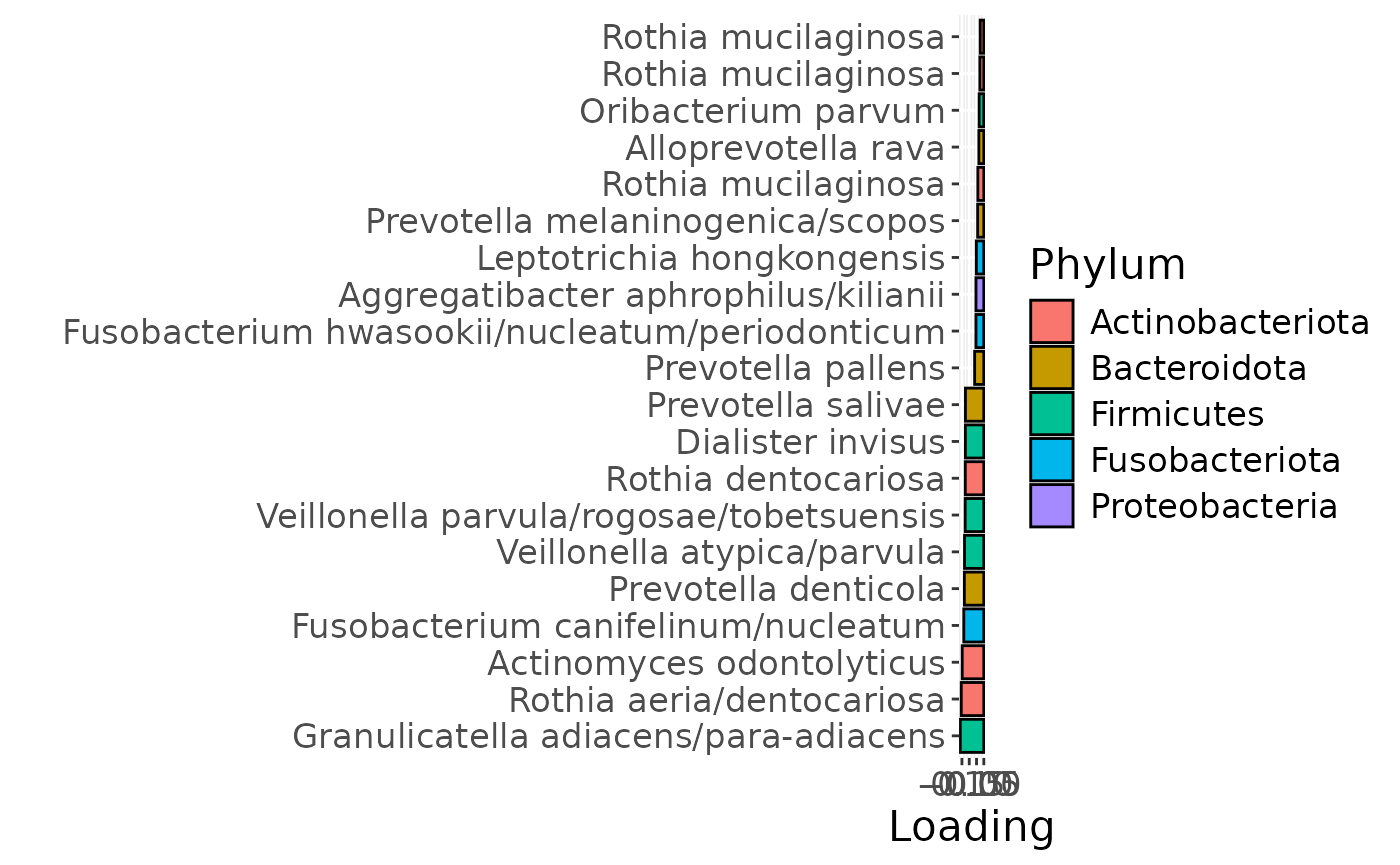
g2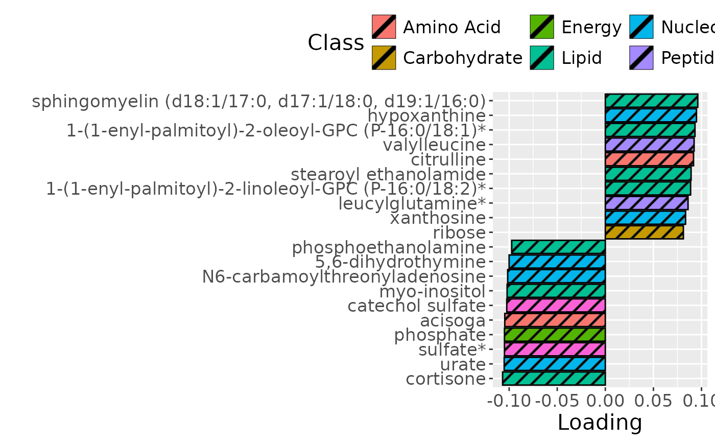
a = processedTongue$mode3 %>%
  mutate(Comp = acmtf_model$Fac[[3]][,3], day=c(-14,0,2,5,9,14,21)) %>%
  select(-visit,-status) %>%
  pivot_longer(-day) %>%
  ggplot(aes(x=day,y=value)) +
  annotate(geom = "rect", xmin = 0, xmax = 14, ymin = -Inf, ymax = Inf, fill = "red", colour = "black", alpha=0.25) +
  geom_line() +
  geom_point() +
  theme(legend.position="none") +
  xlab("Time point [days]") +
  ylab("Loading") +
  ylim(0,1)


b = processedLowling$mode3 %>%
  mutate(Comp = acmtf_model$Fac[[5]][,3], day=c(-14,0,2,5,9,14,21)) %>%
  select(-visit,-status) %>%
  pivot_longer(-day) %>%
  ggplot(aes(x=day,y=value)) +
  annotate(geom = "rect", xmin = 0, xmax = 14, ymin = -Inf, ymax = Inf, fill = "red", colour = "black", alpha=0.25) +
  geom_line() +
  geom_point() +
  theme(legend.position="none") +
  xlab("Time point [days]") +
  ylab("Loading") +
  ylim(0,1)


c = processedLowinter$mode3 %>%
  mutate(Component_1 = -1*acmtf_model$Fac[[7]][,3], day=c(-14,0,2,5,9,14,21)) %>%
  select(-visit,-status) %>%
  pivot_longer(-day) %>%
  ggplot(aes(x=day,y=value)) +
  annotate(geom = "rect", xmin = 0, xmax = 14, ymin = -Inf, ymax = Inf, fill = "red", colour = "black", alpha=0.25) +
  geom_line() +
  geom_point() +
  theme(legend.position="none") +
  xlab("Time point [days]") +
  ylab("Loading") +
  ylim(0,1)

d = processedUpling$mode3 %>%
  mutate(Component_1 = -1*acmtf_model$Fac[[9]][,3], day=c(-14,0,2,5,9,14,21)) %>%
  ggplot(aes(x=day,y=Component_1)) +
  annotate(geom = "rect", xmin = 0, xmax = 14, ymin = -Inf, ymax = Inf, fill = "red", colour = "black", alpha=0.25) +
  geom_line() +
  geom_point() +
  theme(legend.position="none") +
  xlab("Time point [days]") +
  ylab("Loading") +
  ylim(0,1)

e = processedUpinter$mode3 %>%
  mutate(Component_1 = acmtf_model$Fac[[11]][,3], day=c(-14,0,2,5,9,14,21)) %>%
  ggplot(aes(x=day,y=Component_1)) +
  annotate(geom = "rect", xmin = 0, xmax = 14, ymin = -Inf, ymax = Inf, fill = "red", colour = "black", alpha=0.25) +
  geom_line() +
  geom_point() +
  theme(legend.position="none") +
  xlab("Time point [days]") +
  ylab("Loading") +
  ylim(0,1)

f = processedSaliva$mode3 %>%
  mutate(Component_1 = -1*acmtf_model$Fac[[13]][,3], day=c(-14,0,2,5,9,14,21)) %>%
  ggplot(aes(x=day,y=Component_1)) +
  annotate(geom = "rect", xmin = 0, xmax = 14, ymin = -Inf, ymax = Inf, fill = "red", colour = "black", alpha=0.25) +
  geom_line() +
  geom_point() +
  theme(legend.position="none") +
  xlab("Time point [days]") +
  ylab("Loading") +
  ylim(-1,1)

g = processedMetabolomics$mode3 %>%
  mutate(Component_1 = -1*acmtf_model$Fac[[15]][,3], day=c(0,2,5,9,14)) %>%
  ggplot(aes(x=day,y=Component_1)) +
  annotate(geom = "rect", xmin = 0, xmax = 14, ymin = -Inf, ymax = Inf, fill = "red", colour = "black", alpha=0.25) +
  geom_line() +
  geom_point() +
  theme(legend.position="none") +
  xlab("Time point [days]") +
  ylab("Loading") +
  ylim(0,1)

a
b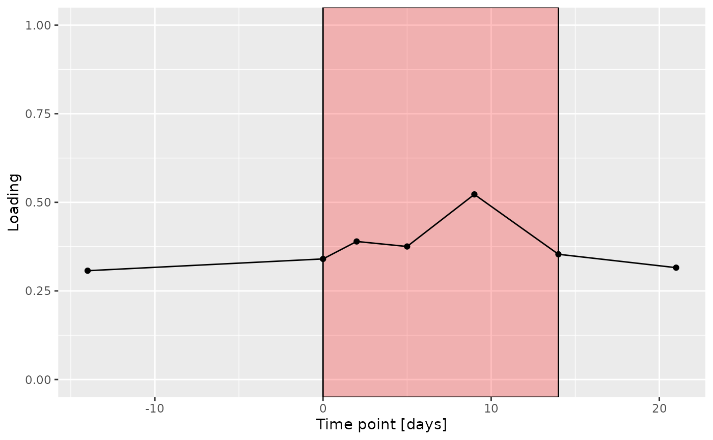
c
d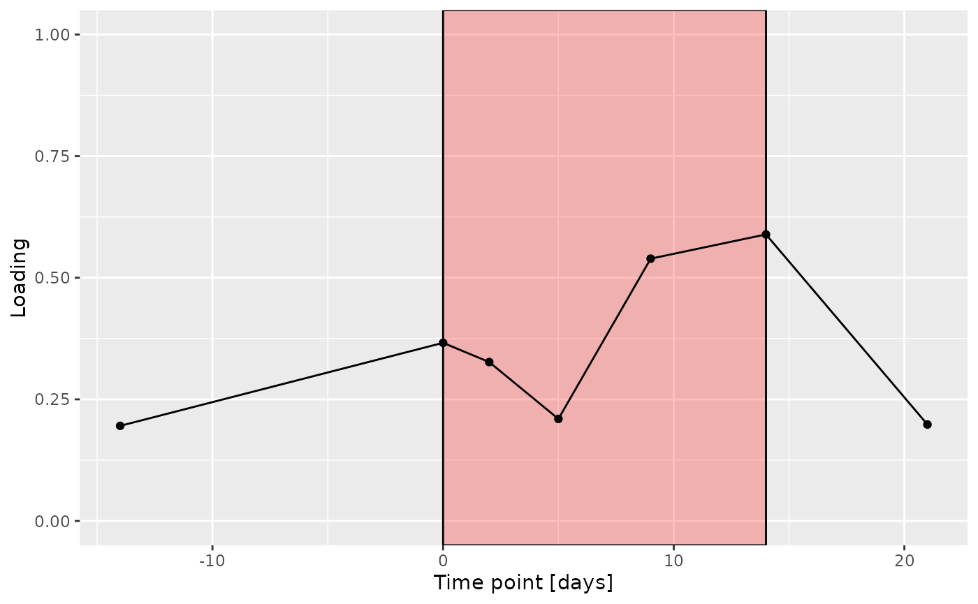
e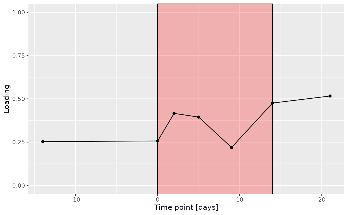
f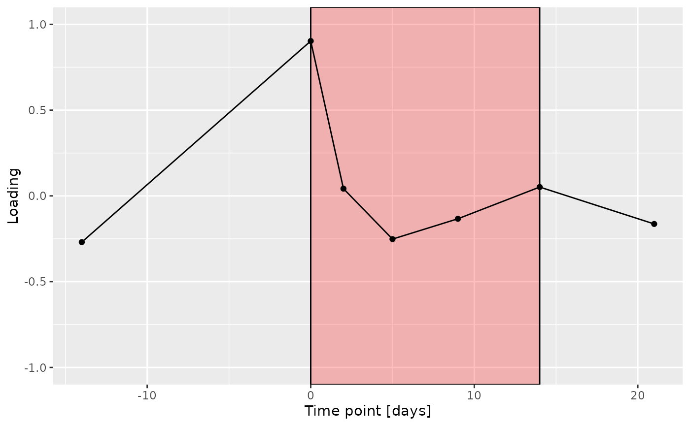
g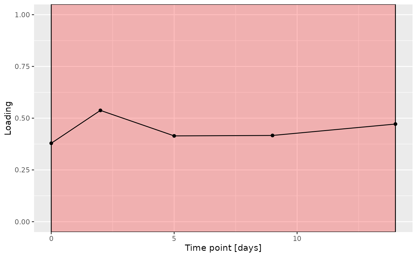
ACMTF-R
Model selection
# Please see the separate R scripts at https://doi.org/10.5281/zenodo.16993009 for the model selection.
acmtfr_model80 = readRDS("./TIFN2/TIFN2_ACMTFR_model_0.8.RDS")
acmtfr_model80$varExp
#> [1] 9.316929 8.047419 3.577750 6.756810 6.790952 6.320588 3.025908
Description
ACMTF-R was next applied to supervise the joint decomposition using the percentage of sites covered in red fluorescent plaque on day 14 (RF%) as dependent variable (y). The model selection procedure revealed that two components were optimal for pi=0.9, based on high and stable FMS random across datasets, FMS CV values greater than 0.9, and only a marginal increase in RMSECV compared to one component. For pi=0.85, 0.8, and 0.5, one component was chosen, as higher-component models showed sharply declining FMS random and FMS CV scores, suggesting poor model stability. Subsequently, the one-component ACMTF-R model using pi=0.80 was selected for further interpretation due to balancing explaining the independent data and predicting y. This model explained 9.3%, 8.1%, 3.6%, 6.8%, 6.8%, 6.3%, 3.0% and 52.3% of the variation in the tongue, lower jaw lingual, lower jaw interproximal, upper jaw lingual, upper jaw interproximal, salivary microbiome, salivary metabolome, and y, respectively.
The Lambda-matrix of the model revealed that the component was predominantly local to the tongue and lower jaw lingual microbiomes, with moderate contributions from the upper jaw lingual, upper jaw interproximal, and salivary microbiome blocks. As expected, MLR analysis revealed that the component was exclusively associated with RF%.
lambda = abs(acmtfr_model80$Fac[[16]])
colnames(lambda) = paste0("C", 1)

lambda %>%
  as_tibble() %>%
  mutate(block=c("tongue", "lowling", "lowinter", "upling", "upinter", "saliva", "metab")) %>%
  mutate(block=factor(block, levels=c("tongue", "lowling", "lowinter", "upling", "upinter", "saliva", "metab"))) %>%
  pivot_longer(-block) %>%
  ggplot(aes(x=as.factor(name),y=value,fill=as.factor(block))) +
  geom_bar(stat="identity",position=position_dodge(),col="black") +
  xlab("ACMTF-R component number") +
  ylab(expression(lambda)) +
  scale_x_discrete(labels=1:3) +
  scale_fill_manual(name="Dataset",values = hue_pal()(7),labels=c("Tongue", "Lower jaw, lingual", "Lower jaw, interproximal", "Upper jaw, lingual", "Upper jaw, interproximal", "Salivary microbiome", "Salivary metabolome")) +
  theme(legend.position="top")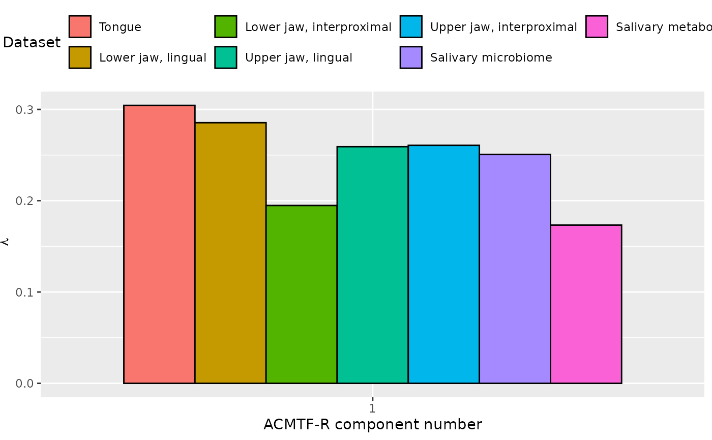
testMetadata(acmtfr_model80, 1, processedTongue)
#>             Term   Estimate                                          CI
#> 1  plaquepercent  -2.353174  -0.00656449861760044 – 0.00185815139043573
#> 2    bomppercent  -2.345146 -0.00492132427908455 – 0.000231031951626678
#> 3 Area_delta_R30 -15.278510   -0.0204756794088214 – -0.0100813405804632
#> 4         gender -72.149196     -0.145433613790882 – 0.0011352227246296
#> 5            age  -1.139687  -0.00765533504288667 – 0.00537596106673432
#>        P_value     P_adjust
#> 1 2.640812e-01 3.301015e-01
#> 2 7.302173e-02 1.217029e-01
#> 3 9.298468e-07 4.649234e-06
#> 4 5.345353e-02 1.217029e-01
#> 5 7.244329e-01 7.244329e-01
# Pi = 0.8
temp = list()
temp$Fac = acmtfr_model80$Fac[c(1,2,3)]
testFeatures(temp, processedTongue, 1, "Area_delta_R30") # flip
#> Joining with `by = join_by(subject, RFgroup)`
#> Joining with `by = join_by(subject, age, gender)`
#> [1] "Positive loadings:"
#>      Area_delta_R30
#> [1,]     -0.7233091
#> [1] "Negative loadings:"
#>      Area_delta_R30
#> [1,]      0.7233091
a = plotFeatures(processedTongue$mode2, temp, 1, flip=TRUE) + scale_fill_manual(values=phylum_colors[-c(3,7)])

temp = list()
temp$Fac = acmtfr_model80$Fac[c(1,4,5)]
testFeatures(temp, processedLowling, 1, "Area_delta_R30") # flip
#> Joining with `by = join_by(subject, RFgroup)`
#> Joining with `by = join_by(subject, age, gender)`
#> [1] "Positive loadings:"
#>      Area_delta_R30
#> [1,]     -0.7233091
#> [1] "Negative loadings:"
#>      Area_delta_R30
#> [1,]      0.7233091
b = plotFeatures(processedLowling$mode2, temp, 1, flip=TRUE) + scale_fill_manual(values=phylum_colors[-7])

temp = list()
temp$Fac = acmtfr_model80$Fac[c(1,6,7)]
testFeatures(temp, processedLowinter, 1, "Area_delta_R30") # flip
#> Joining with `by = join_by(subject, RFgroup)`
#> Joining with `by = join_by(subject, age, gender)`
#> [1] "Positive loadings:"
#>      Area_delta_R30
#> [1,]     -0.7233091
#> [1] "Negative loadings:"
#>      Area_delta_R30
#> [1,]      0.7233091
c = plotFeatures(processedLowinter$mode2, temp, 1, flip=TRUE) + scale_fill_manual(values=phylum_colors[-c(3,7)])

temp = list()
temp$Fac = acmtfr_model80$Fac[c(1,8,9)]
testFeatures(temp, processedUpling, 1, "Area_delta_R30")
#> Joining with `by = join_by(subject, RFgroup)`
#> Joining with `by = join_by(subject, age, gender)`
#> [1] "Positive loadings:"
#>      Area_delta_R30
#> [1,]      0.7233091
#> [1] "Negative loadings:"
#>      Area_delta_R30
#> [1,]     -0.7233091
d = plotFeatures(processedUpling$mode2, temp, 1, flip=FALSE) + scale_fill_manual(values=phylum_colors[-c(3,7)])

temp = list()
temp$Fac = acmtfr_model80$Fac[c(1,10,11)]
testFeatures(temp, processedUpinter, 1, "Area_delta_R30") # flip
#> Joining with `by = join_by(subject, RFgroup)`
#> Joining with `by = join_by(subject, age, gender)`
#> [1] "Positive loadings:"
#>      Area_delta_R30
#> [1,]     -0.7233091
#> [1] "Negative loadings:"
#>      Area_delta_R30
#> [1,]      0.7233091
e = plotFeatures(processedUpinter$mode2, temp, 1, flip=TRUE) + scale_fill_manual(values=phylum_colors[-c(3,7)])

temp = list()
temp$Fac = acmtfr_model80$Fac[c(1,12,13)]
testFeatures(temp, processedSaliva, 1, "Area_delta_R30") # flip
#> Joining with `by = join_by(subject, RFgroup)`
#> Joining with `by = join_by(subject, age, gender)`
#> [1] "Positive loadings:"
#>      Area_delta_R30
#> [1,]     -0.7233091
#> [1] "Negative loadings:"
#>      Area_delta_R30
#> [1,]      0.7233091
f = plotFeatures(processedSaliva$mode2, temp, 1, flip=TRUE) + scale_fill_manual(values=phylum_colors[-c(3,7)])

# Metab
temp = list()
temp$Fac = acmtfr_model80$Fac[c(1,14,15)]
testFeatures(temp, processedMetabolomics, 1, "Area_delta_R30") # no flip
#> Joining with `by = join_by(subject, RFgroup)`
#> Joining with `by = join_by(subject, age, gender)`
#> [1] "Positive loadings:"
#>      Area_delta_R30
#> [1,]      0.7233091
#> [1] "Negative loadings:"
#>      Area_delta_R30
#> [1,]     -0.7233091

df = processedMetabolomics$mode2 %>% mutate(Component_2 = acmtfr_model80$Fac[[14]][,1]) %>% arrange(Component_2) %>% mutate(index=1:nrow(.))
df = rbind(df %>% head(n=10), df %>% tail(n=10))

g = df %>%
  ggplot(aes(x = Component_2, y = as.factor(index),
             fill = as.factor(Type),
             pattern = as.factor(Type))) +
  geom_bar_pattern(stat = "identity",
                   colour = "black",
                   pattern = "stripe",
                   pattern_fill = "black",
                   pattern_density = 0.2,
                   pattern_spacing = 0.05,
                   pattern_angle = 45,
                   pattern_size = 0.2) +
  scale_y_discrete(labels = df$Name) +
  xlab("Loading") +
  ylab("") +
  guides(fill = guide_legend(title = "Class"),
         pattern = "none") +
  theme(text = element_text(size = 16),
        legend.position = "top")

a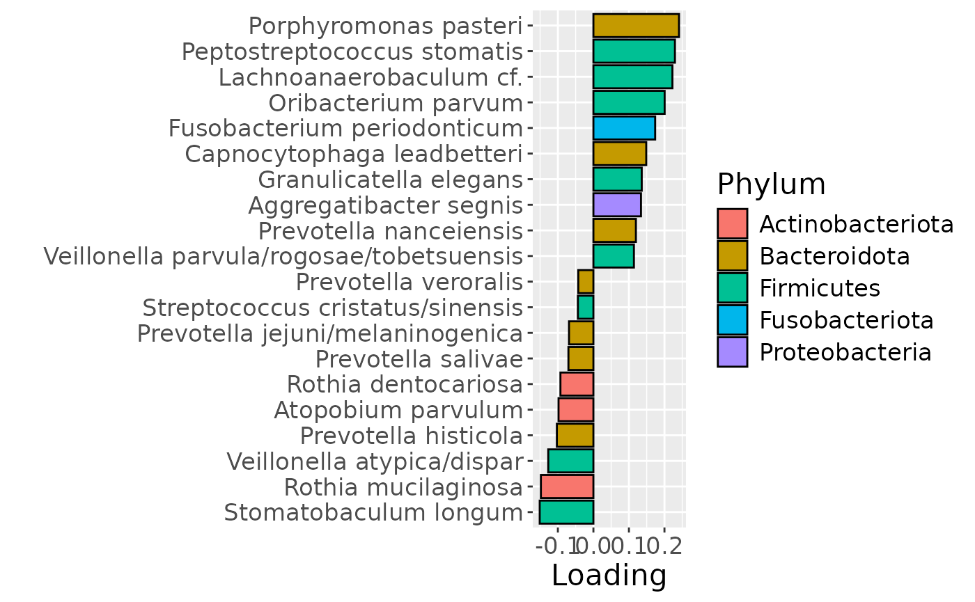
b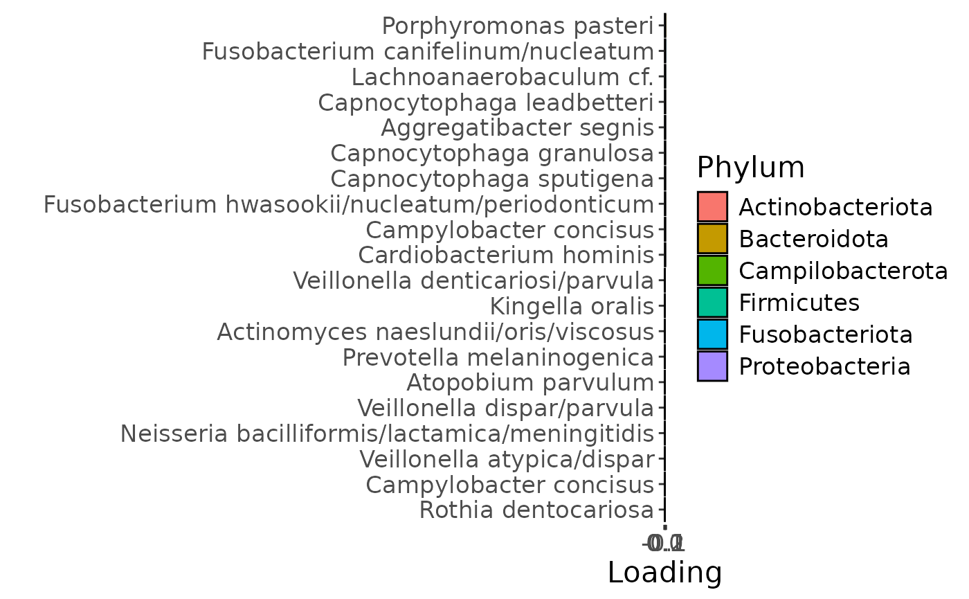
c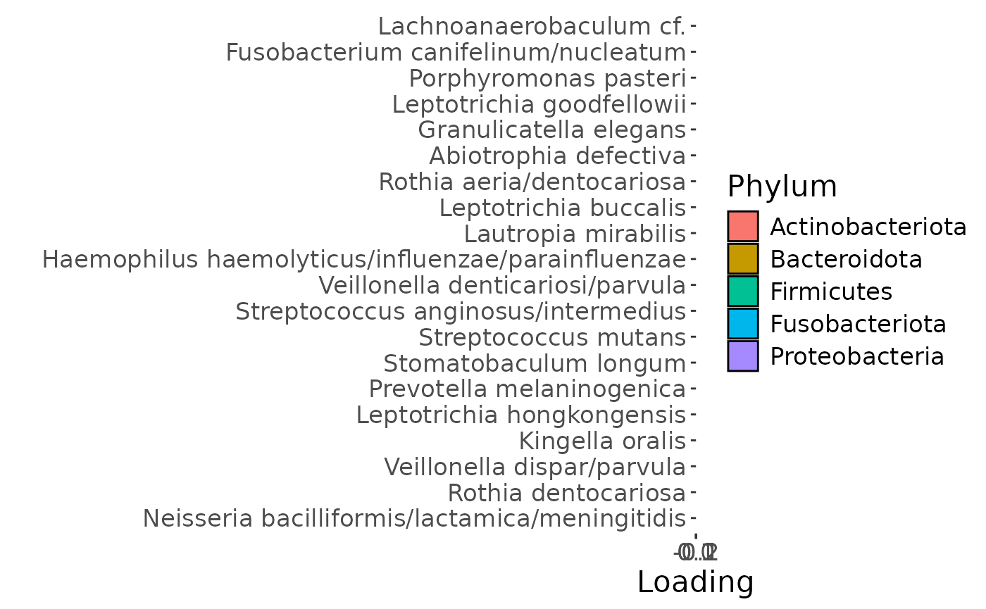
d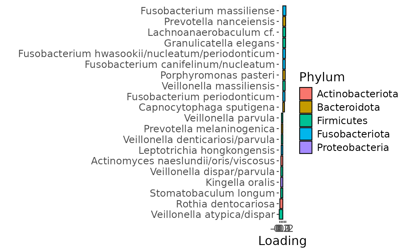
e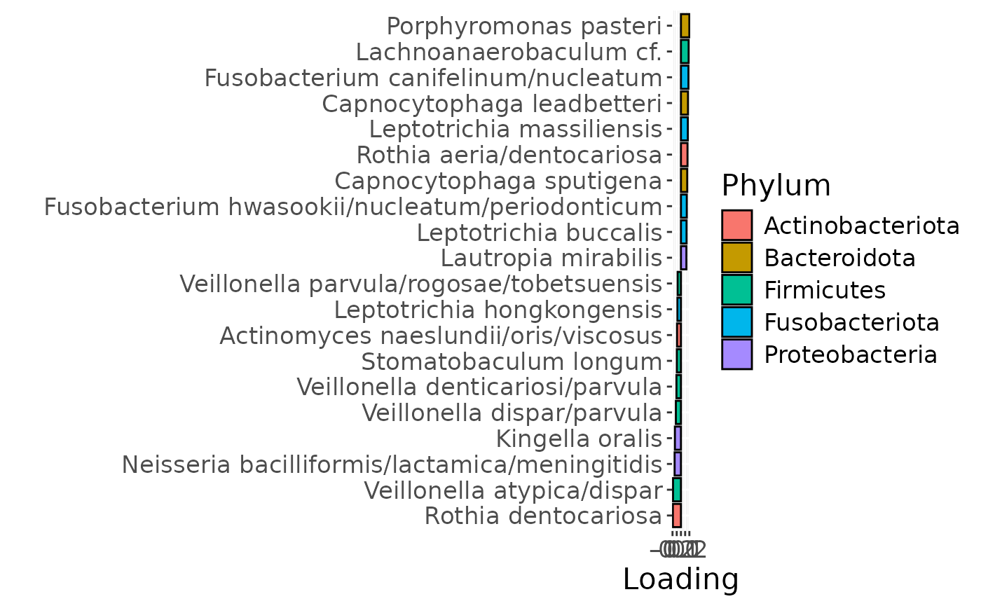
f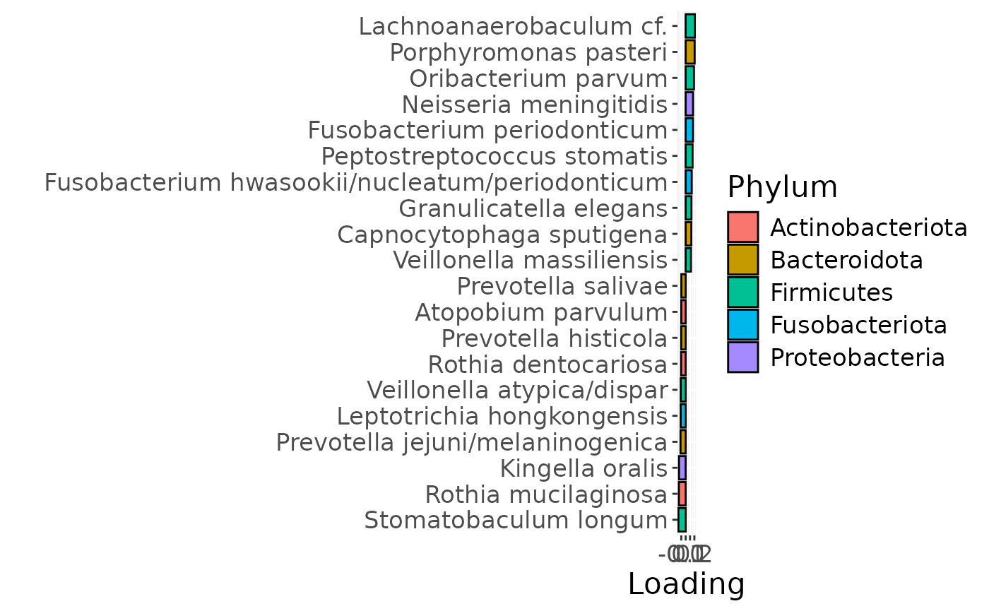
g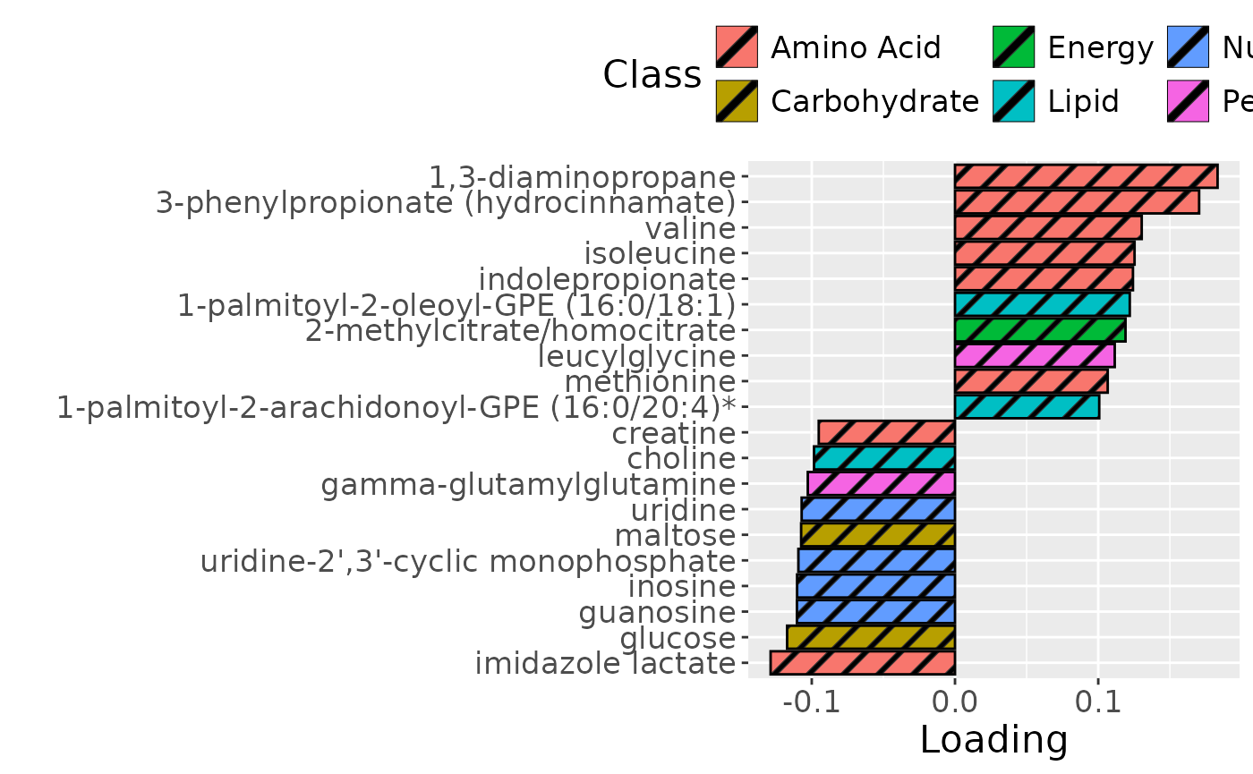
a = processedTongue$mode3 %>%
  mutate(Comp = acmtfr_model80$Fac[[3]][,1], day=c(-14,0,2,5,9,14,21)) %>%
  select(-visit,-status) %>%
  pivot_longer(-day) %>%
  ggplot(aes(x=day,y=value)) +
  annotate(geom = "rect", xmin = 0, xmax = 14, ymin = -Inf, ymax = Inf, fill = "red", colour = "black", alpha=0.25) +
  geom_line() +
  geom_point() +
  theme(legend.position="none") +
  xlab("Time point [days]") +
  ylab("Loading") +
  ylim(0,1)

b = processedLowling$mode3 %>%
  mutate(Component_1 = acmtfr_model80$Fac[[5]][,1], day=c(-14,0,2,5,9,14,21)) %>%
  ggplot(aes(x=day,y=Component_1)) +
  annotate(geom = "rect", xmin = 0, xmax = 14, ymin = -Inf, ymax = Inf, fill = "red", colour = "black", alpha=0.25) +
  geom_line() +
  geom_point() +
  theme(legend.position="none") +
  xlab("Time point [days]") +
  ylab("Loading") +
  ylim(0,1)

c = processedLowinter$mode3 %>%
  mutate(Component_1 = acmtfr_model80$Fac[[7]][,1], day=c(-14,0,2,5,9,14,21)) %>%
  ggplot(aes(x=day,y=Component_1)) +
  annotate(geom = "rect", xmin = 0, xmax = 14, ymin = -Inf, ymax = Inf, fill = "red", colour = "black", alpha=0.25) +
  geom_line() +
  geom_point() +
  theme(legend.position="none") +
  xlab("Time point [days]") +
  ylab("Loading") +
  ylim(0,1)

d = processedUpling$mode3 %>%
  mutate(Component_1 = -1*acmtfr_model80$Fac[[9]][,1], day=c(-14,0,2,5,9,14,21)) %>%
  ggplot(aes(x=day,y=Component_1)) +
  annotate(geom = "rect", xmin = 0, xmax = 14, ymin = -Inf, ymax = Inf, fill = "red", colour = "black", alpha=0.25) +
  geom_line() +
  geom_point() +
  theme(legend.position="none") +
  xlab("Time point [days]") +
  ylab("Loading") +
  ylim(0,1)

e = processedUpinter$mode3 %>%
  mutate(Component_1 = acmtfr_model80$Fac[[11]][,1], day=c(-14,0,2,5,9,14,21)) %>%
  ggplot(aes(x=day,y=Component_1)) +
  annotate(geom = "rect", xmin = 0, xmax = 14, ymin = -Inf, ymax = Inf, fill = "red", colour = "black", alpha=0.25) +
  geom_line() +
  geom_point() +
  theme(legend.position="none") +
  xlab("Time point [days]") +
  ylab("Loading") +
  ylim(0,1)

f = processedSaliva$mode3 %>%
  mutate(Comp = acmtfr_model80$Fac[[13]][,1], day=c(-14,0,2,5,9,14,21)) %>%
  select(-visit,-status) %>%
  pivot_longer(-day) %>%
  ggplot(aes(x=day,y=value)) +
  annotate(geom = "rect", xmin = 0, xmax = 14, ymin = -Inf, ymax = Inf, fill = "red", colour = "black", alpha=0.25) +
  geom_line() +
  geom_point() +
  theme(legend.position="none") +
  xlab("Time point [days]") +
  ylab("Loading") +
  ylim(0,1)

g = processedMetabolomics$mode3 %>%
  mutate(Comp = acmtfr_model80$Fac[[15]][,1], day=c(0,2,5,9,14)) %>%
  select(-visit,-status) %>%
  pivot_longer(-day) %>%
  ggplot(aes(x=day,y=-1*value)) +
  annotate(geom = "rect", xmin = 0, xmax = 14, ymin = -Inf, ymax = Inf, fill = "red", colour = "black", alpha=0.25) +
  geom_line() +
  geom_point() +
  theme(legend.position="none") +
  xlab("Time point [days]") +
  ylab("Loading") +
  ylim(0,1)

a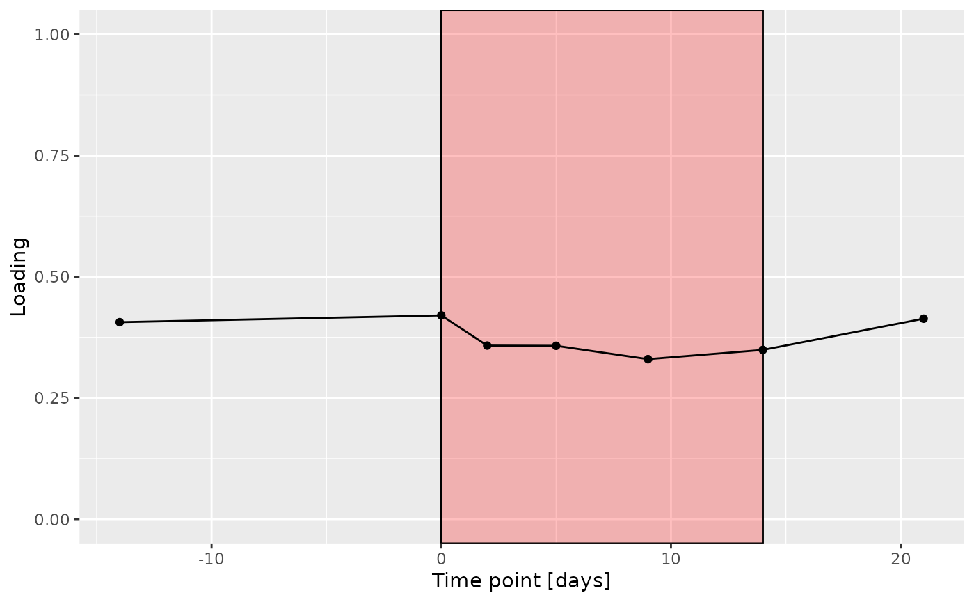
b
c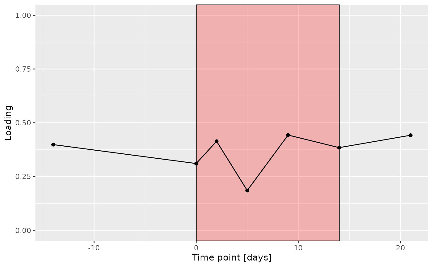
d
e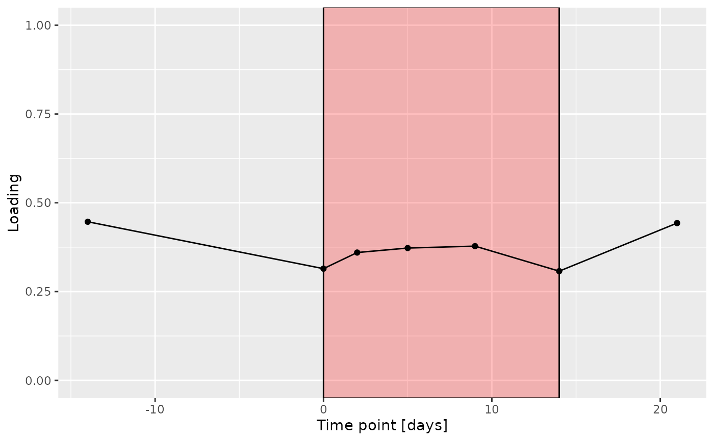
f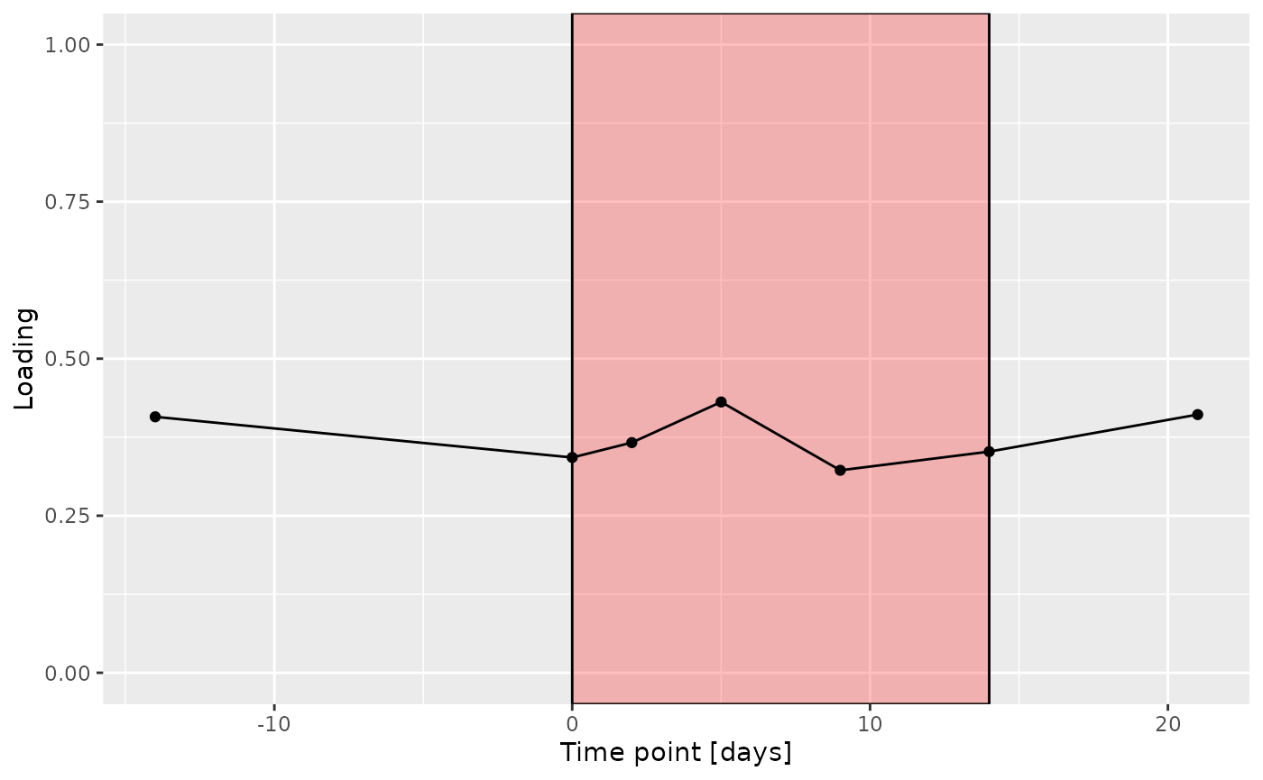
g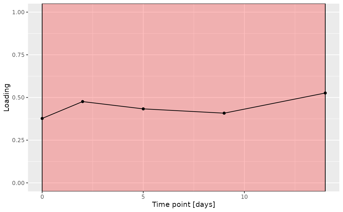 Across the microbiome datasets, consistently positively loaded taxa
including Aggregatibacter, Fusobacterium, Leptotrichia,
Peptostreptococcus, Porphyromonas, and Fusobacterium nucleatum were
enriched in high responders and depleted in low responders. Conversely,
consistently negatively loaded taxa including Kingella, Lautropia,
Prevotella, Rothia, Streptococcus, and Veillonella were enriched in low
responders and enriched in high responders. Overall, inter-subject
differences due to RF% remained relatively constant, with a small
increase during the intervention.
Across the microbiome datasets, consistently positively loaded taxa
including Aggregatibacter, Fusobacterium, Leptotrichia,
Peptostreptococcus, Porphyromonas, and Fusobacterium nucleatum were
enriched in high responders and depleted in low responders. Conversely,
consistently negatively loaded taxa including Kingella, Lautropia,
Prevotella, Rothia, Streptococcus, and Veillonella were enriched in low
responders and enriched in high responders. Overall, inter-subject
differences due to RF% remained relatively constant, with a small
increase during the intervention.
Higher RF% was associated with elevated levels of amino acids, including valine, isoleucine, and methionine. Conversely, individuals with lower RF% exhibited higher levels of peptides (e.g., uridine, inosine, and guanosine) and some carbohydrates (e.g., glucose and maltose). The time mode loadings indicate that inter-subject differences due to the intervention remained relatively constant.