GOHTRANS: gender-affirming hormone therapy
2025-08-31
Source:vignettes/articles/GOHTRANS.Rmd
GOHTRANS.RmdIntroduction
This article presents the NPLS results of the GOHTRANS dataset discussed in Chapter 6 of my dissertation.
Preamble
library(dplyr)
#>
#> Attaching package: 'dplyr'
#> The following objects are masked from 'package:stats':
#>
#>     filter, lag
#> The following objects are masked from 'package:base':
#>
#>     intersect, setdiff, setequal, union
library(tidyr)
library(parafac4microbiome)
library(NPLStoolbox)
library(CMTFtoolbox)
#>
#> Attaching package: 'CMTFtoolbox'
#> The following object is masked from 'package:NPLStoolbox':
#>
#>     npred
#> The following objects are masked from 'package:parafac4microbiome':
#>
#>     fac_to_vect, reinflateFac, reinflateTensor, vect_to_fac
library(ggplot2)
library(ggpubr)
library(readr)
library(stringr)
ph_BOMP = read_delim("./GOHTRANS/GOH-TRANS_export_20240205.csv",
                     delim = ";", escape_double = FALSE, trim_ws = TRUE) %>% as_tibble()
#> Rows: 42 Columns: 347
#> ── Column specification ────────────────────────────────────────────────────────
#> Delimiter: ";"
#> chr (104): Participant Status, Site Abbreviation, Participant Creation Date,...
#> dbl (243): Participant Id, pat_genderID, Age, Informed_consent#Yes, Informed...
#>
#> ℹ Use `spec()` to retrieve the full column specification for this data.
#> ℹ Specify the column types or set `show_col_types = FALSE` to quiet this message.

df1 = ph_BOMP %>% select(`Participant Id`, starts_with("5.")) %>% mutate(subject = 1:42, numTeeth = `5.1|Number of teeth`, DMFT = `5.2|DMFT`, numBleedingSites = `5.3|Bleeding sites`, boppercent = `5.4|BOP%`, DPSI = `5.5|DPSI`, pH = `5.8|pH`) %>% select(subject, numTeeth, DMFT, numBleedingSites, boppercent, DPSI, pH)
df2 = ph_BOMP %>% select(`Participant Id`, starts_with("12.")) %>% mutate(subject = 1:42, numTeeth = `12.1|Number of teeth`, DMFT = `12.2|DMFT`, numBleedingSites = `12.3|Bleeding sites`, boppercent = `12.4|BOP%`, DPSI = `12.5|DPSI`, pH = `12.8|pH`) %>% select(subject, numTeeth, DMFT, numBleedingSites, boppercent, DPSI, pH)
df3 = ph_BOMP %>% select(`Participant Id`, starts_with("19.")) %>% mutate(subject = 1:42, numTeeth = `19.1|Number of teeth`, DMFT = `19.2|DMFT`, numBleedingSites = `19.3|Bleeding sites`, boppercent = `19.4|BOP%`, DPSI = `19.5|DPSI`, pH = `19.8|pH`) %>% select(subject, numTeeth, DMFT, numBleedingSites, boppercent, DPSI, pH)
df4 = ph_BOMP %>% select(`Participant Id`, starts_with("26.")) %>% mutate(subject = 1:42, numTeeth = `26.1|Number of teeth`, DMFT = `26.2|DMFT`, numBleedingSites = `26.3|Bleeding sites`, boppercent = `26.4|BOP%`, DPSI = `26.5|DPSI`, pH = `26.8|pH`) %>% select(subject, numTeeth, DMFT, numBleedingSites, boppercent, DPSI, pH)

otherMeta = rbind(df1, df2, df3, df4) %>% as_tibble() %>% mutate(newTimepoint = rep(c(0,3,6,12), each=42))
otherMeta = otherMeta %>% select(subject, newTimepoint, boppercent)
otherMeta[otherMeta$boppercent < 0 & !is.na(otherMeta$boppercent), "boppercent"] = NA

saliva_sampleMeta = read.csv("./GOHTRANS/sampleInfo_fixed.csv", sep=" ") %>% as_tibble() %>% select(subject, GenderID, Age, newTimepoint)

# CODS XI
df = read.csv("./GOHTRANS/CODS_XI.csv")
df = df[1:40,1:10] %>% as_tibble() %>% filter(Participant_code %in% saliva_sampleMeta$subject)

CODS = df %>% select(Participant_code, CODS_BASELINE, CODS_3_MONTHS, CODS_6_MONTHS, CODS_12_MONTHS) %>% pivot_longer(-Participant_code) %>% mutate(timepoint = NA)
CODS[CODS$name == "CODS_BASELINE", "timepoint"] = 0
CODS[CODS$name == "CODS_3_MONTHS", "timepoint"] = 3
CODS[CODS$name == "CODS_6_MONTHS", "timepoint"] = 6
CODS[CODS$name == "CODS_12_MONTHS", "timepoint"] = 12
CODS[CODS$value == -99, "value"] = NA
CODS = CODS %>% mutate(subject = Participant_code, newTimepoint = timepoint, CODS = value) %>% select(-Participant_code, -name, -value, -timepoint)

XI = df %>% select(Participant_code, XI_BASELINE, XI_3_MONTHS, XI_6_MONTHS, XI_12_MONTHS) %>% pivot_longer(-Participant_code) %>% mutate(timepoint = NA)
XI[XI$name == "XI_BASELINE", "timepoint"] = 0
XI[XI$name == "XI_3_MONTHS", "timepoint"] = 3
XI[XI$name == "XI_6_MONTHS", "timepoint"] = 6
XI[XI$name == "XI_12_MONTHS", "timepoint"] = 12
XI[XI$value == -99, "value"] = NA
XI = XI %>% mutate(subject = Participant_code, newTimepoint = timepoint, XI = value) %>% select(-Participant_code, -name, -value, -timepoint)

df = otherMeta %>% left_join(CODS) %>% left_join(XI) %>% select(subject, newTimepoint, boppercent, CODS, XI) %>% filter(newTimepoint != "NA")
#> Joining with `by = join_by(subject, newTimepoint)`
#> Joining with `by = join_by(subject, newTimepoint)`

meta = df %>% left_join(otherMeta) %>% left_join(saliva_sampleMeta) %>% filter(newTimepoint==12) %>% unique() %>% select(-newTimepoint)
#> Joining with `by = join_by(subject, newTimepoint, boppercent)`
#> Joining with `by = join_by(subject, newTimepoint)`
meta[meta < 0] <- NA

newBOP = residuals(lm(boppercent ~ GenderID + Age + CODS + XI, data=meta, na.action=na.exclude))
newCODS= residuals(lm(CODS ~ boppercent + GenderID + Age + XI, data=meta, na.action=na.exclude))
newXI = residuals(lm(XI ~ boppercent + GenderID + Age + CODS, data=meta, na.action=na.exclude))

meta = meta %>% mutate(boppercent = newBOP, CODS = newCODS, XI = newXI)
prepMetadata = function(model, metadata){
  longA = parafac4microbiome::transformPARAFACloadings(model$Fac, 2, moreOutput = TRUE)$F
  df = longA %>% as_tibble() %>% mutate(subject=as.integer(rep(metadata$mode1$subject, each=nrow(metadata$mode3))), newTimepoint = rep(metadata$mode3$newTimepoint, nrow(metadata$mode1))) %>% left_join(Cornejo2025$Blood_hormones) %>% left_join(Cornejo2025$Clinical_measurements)

  newTesto = residuals(lm(Free_testosterone_Vermeulen_pmol_L ~ Estradiol_pmol_ml + LH_U_L + SHBG_nmol_L + boppercent + pH + GenderID + Age, data=df, na.action=na.exclude))
  newEstra = residuals(lm(Estradiol_pmol_ml ~ Free_testosterone_Vermeulen_pmol_L + LH_U_L + SHBG_nmol_L + boppercent + pH + GenderID + Age, data=df, na.action=na.exclude))
  newLH = residuals(lm(LH_U_L ~ Free_testosterone_Vermeulen_pmol_L + Estradiol_pmol_ml + SHBG_nmol_L + boppercent + pH + GenderID + Age, data=df, na.action=na.exclude))
  newSHBG = residuals(lm(SHBG_nmol_L ~ Free_testosterone_Vermeulen_pmol_L + Estradiol_pmol_ml + LH_U_L + boppercent + pH + GenderID + Age, data=df, na.action=na.exclude))
  newBOP = residuals(lm(boppercent ~ Free_testosterone_Vermeulen_pmol_L + Estradiol_pmol_ml + LH_U_L + SHBG_nmol_L + pH + GenderID + Age, data=df, na.action=na.exclude))
  newPH = residuals(lm(pH ~ Free_testosterone_Vermeulen_pmol_L + Estradiol_pmol_ml + LH_U_L + SHBG_nmol_L + boppercent + GenderID + Age, data=df, na.action=na.exclude))

  df$Free_testosterone_Vermeulen_pmol_L = newTesto
  df$Estradiol_pmol_ml = newEstra
  df$LH_U_L = newLH
  df$SHBG_nmol_L = newSHBG
  df$boppercent = newBOP
  df$pH = newPH
  df$GenderID = as.numeric(as.factor(df$GenderID))

  return(df)
}

clinical_metadata = NPLStoolbox::Cornejo2025$Clinical_measurements$mode1 %>% mutate(BOP = NPLStoolbox::Cornejo2025$Clinical_measurements$data[,1,2], CODS = NPLStoolbox::Cornejo2025$Clinical_measurements$data[,2,2], XI = NPLStoolbox::Cornejo2025$Clinical_measurements$data[,3,2]) %>% left_join(NPLStoolbox::Cornejo2025$Subject_metadata %>% mutate(subject = as.character(subject)))
#> Joining with `by = join_by(subject, GenderID)`

testMetadata = function(model, comp, metadata){
  transformedSubjectLoadings = model$Fac[[1]][,comp]
  transformedSubjectLoadings = transformedSubjectLoadings / norm(transformedSubjectLoadings, "2")

  metadata = metadata$mode1 %>% left_join(clinical_metadata) %>% mutate(GenderID = as.numeric(as.factor(GenderID))-1)

  result = lm(transformedSubjectLoadings ~ GenderID + Age + BOP + CODS + XI, data=metadata)

  # Extract coefficients and confidence intervals
  coef_estimates <- summary(result)$coefficients
  conf_intervals <- confint(result)

  # Remove intercept
  coef_estimates <- coef_estimates[rownames(coef_estimates) != "(Intercept)", ]
  conf_intervals <- conf_intervals[rownames(conf_intervals) != "(Intercept)", ]

  # Combine into a clean data frame
  summary_table <- data.frame(
    Term     = rownames(coef_estimates),
    Estimate = coef_estimates[, "Estimate"] * 1e3,
    CI       = paste0(
                 conf_intervals[, 1], " – ",
                 conf_intervals[, 2]
               ),
    P_value  = coef_estimates[, "Pr(>|t|)"],
    P_adjust = p.adjust(coef_estimates[, "Pr(>|t|)"], "BH"),
    row.names = NULL
  )

  return(summary_table)
}
processedTongue = processDataCube(NPLStoolbox::Cornejo2025$Tongue_microbiome, sparsityThreshold = 0.5, considerGroups=TRUE, groupVariable="GenderID", CLR=TRUE, centerMode=1, scaleMode=2)
processedSaliva = processDataCube(NPLStoolbox::Cornejo2025$Salivary_microbiome, sparsityThreshold = 0.5, considerGroups=TRUE, groupVariable="GenderID", CLR=TRUE, centerMode=1, scaleMode=2)

processedCytokines = NPLStoolbox::Cornejo2025$Salivary_cytokines
processedCytokines$data = log(processedCytokines$data + 0.1300)
# Remove subject 1, 18, 19, and 27 due to being an outlier
processedCytokines$data = processedCytokines$data[-c(1,9,10,19),,]
processedCytokines$mode1 = processedCytokines$mode1[-c(1,9,10,19),]
processedCytokines$data = multiwayCenter(processedCytokines$data, 1)
processedCytokines$data = multiwayScale(processedCytokines$data, 2)

processedBiochemistry = NPLStoolbox::Cornejo2025$Salivary_biochemistry
processedBiochemistry$data = log(processedBiochemistry$data)
processedBiochemistry$data = multiwayCenter(processedBiochemistry$data, 1)
processedBiochemistry$data = multiwayScale(processedBiochemistry$data, 2)

processedHormones = NPLStoolbox::Cornejo2025$Circulatory_hormones
processedHormones$data = log(processedHormones$data)
processedHormones$data = multiwayCenter(processedHormones$data, 1)
processedHormones$data = multiwayScale(processedHormones$data, 2)
deltaT = NPLStoolbox::Cornejo2025$Circulatory_hormones$data[,1,2] - NPLStoolbox::Cornejo2025$Circulatory_hormones$data[,1,1]
outcome = processedHormones$mode1 %>% mutate(deltaT = deltaT) %>% filter(deltaT != "NA")
processedTongue = processDataCube(NPLStoolbox::Cornejo2025$Tongue_microbiome, sparsityThreshold = 0.5, considerGroups=TRUE, groupVariable="GenderID", CLR=TRUE, centerMode=FALSE, scaleMode=FALSE)
mask = processedTongue$mode1$subject %in% outcome$subject
processedTongue$mode1 = processedTongue$mode1[mask,]
processedTongue$data = processedTongue$data[mask,,]
processedTongue$data = multiwayCenter(processedTongue$data, 1)
processedTongue$data = multiwayScale(processedTongue$data, 2)

processedSaliva = processDataCube(NPLStoolbox::Cornejo2025$Salivary_microbiome, sparsityThreshold = 0.5, considerGroups=TRUE, groupVariable="GenderID", CLR=TRUE, centerMode=1, scaleMode=2)
mask = processedSaliva$mode1$subject %in% outcome$subject
processedSaliva$mode1 = processedSaliva$mode1[mask,]
processedSaliva$data = processedSaliva$data[mask,,]
processedSaliva$data = multiwayCenter(processedSaliva$data, 1)
processedSaliva$data = multiwayScale(processedSaliva$data, 2)

processedCytokines = NPLStoolbox::Cornejo2025$Salivary_cytokines
processedCytokines$data = log(processedCytokines$data + 0.1300)
# Remove subject 1, 18, 19, and 27 due to being an outlier
processedCytokines$data = processedCytokines$data[-c(1,9,10,19),,]
processedCytokines$mode1 = processedCytokines$mode1[-c(1,9,10,19),]
mask = processedCytokines$mode1$subject %in% outcome$subject
processedCytokines$mode1 = processedCytokines$mode1[mask,]
processedCytokines$data = processedCytokines$data[mask,,]
processedCytokines$data = multiwayCenter(processedCytokines$data, 1)
processedCytokines$data = multiwayScale(processedCytokines$data, 2)

processedBiochemistry = NPLStoolbox::Cornejo2025$Salivary_biochemistry
processedBiochemistry$data = log(processedBiochemistry$data)
mask = processedBiochemistry$mode1$subject %in% outcome$subject
processedBiochemistry$mode1 = processedBiochemistry$mode1[mask,]
processedBiochemistry$data = processedBiochemistry$data[mask,,]
processedBiochemistry$data = multiwayCenter(processedBiochemistry$data, 1)
processedBiochemistry$data = multiwayScale(processedBiochemistry$data, 2)
Y = processedTongue$mode1 %>% left_join(outcome) %>% select(deltaT) %>% pull()
#> Joining with `by = join_by(subject, GenderID)`
Ycnt = Y - mean(Y)
Ynorm_tongue = Ycnt / norm(Ycnt, "2")

Y = processedSaliva$mode1 %>% left_join(outcome) %>% select(deltaT) %>% pull()
#> Joining with `by = join_by(subject, GenderID)`
Ycnt = Y - mean(Y)
Ynorm_saliva = Ycnt / norm(Ycnt, "2")

Y = processedCytokines$mode1 %>% left_join(outcome) %>% select(deltaT) %>% pull()
#> Joining with `by = join_by(subject, GenderID)`
Ycnt = Y - mean(Y)
Ynorm_cytokine = Ycnt / norm(Ycnt, "2")

Y = processedBiochemistry$mode1 %>% left_join(outcome) %>% select(deltaT) %>% pull()
#> Joining with `by = join_by(subject, GenderID)`
Ycnt = Y - mean(Y)
Ynorm_biochem = Ycnt / norm(Ycnt, "2")
Tongue microbiome
NPLS was next applied to supervise the decomposition using the difference in free testosterone between baseline and month three of GAHT as the dependent variable (y). The model selection procedure revealed that a one-component NPLS model corresponded to the RMSECV minimum, explaining 5.7% of the variation in X, and 29.2% of the variation in y. The commented code below performs the procedure, and is not rerun here due to computational limitations.
# CV_tongue = NPLStoolbox::ncrossreg(processedTongue$data, Ynorm_tongue, maxNumComponents = 10)
# a=CV_tongue$varExp %>% pivot_longer(-numComponents) %>% ggplot(aes(x=as.factor(numComponents),y=value,col=as.factor(name),group=as.factor(name))) + geom_line() + geom_point() + xlab("Number of components") + ylab("Variance explained (%)") + theme(legend.position="none")
# b=CV_tongue$RMSE %>% ggplot(aes(x=numComponents,y=RMSE)) + geom_line() + geom_point() + xlab("Number of components") + ylab("RMSECV")
# ggarrange(a,b) # 1
# npls_tongue = NPLStoolbox::triPLS1(processedTongue$data, Ynorm_tongue, 1)
npls_tongue = readRDS("./GOHTRANS/NPLS_tongue_deltaT.RDS")

npls_tongue$varExpX
#> [1] 5.746214
npls_tongue$varExpY
#> [1] 29.23862
As expected, MLR analysis revealed that the model captured variation exclusively associated with gender identity.
testMetadata(npls_tongue, 1, processedTongue)
#> Joining with `by = join_by(subject, GenderID)`
#>       Term     Estimate                                        CI    P_value
#> 1 GenderID -146.0032589  -0.266023951164381 – -0.0259825666217627 0.01911011
#> 2      Age   -0.1299597  -0.0135672435837477 – 0.0133073242724576 0.98426614
#> 3      BOP    3.0539354 -0.00483738995653187 – 0.0109452608045115 0.43293306
#> 4     CODS    2.7772659  -0.0106562762659828 – 0.0162108080786144 0.67390326
#> 5       XI    3.3350268  -0.0105643068932559 – 0.0172343605614402 0.62550130
#>     P_adjust
#> 1 0.09555055
#> 2 0.98426614
#> 3 0.84237908
#> 4 0.84237908
#> 5 0.84237908
a = processedTongue$mode1 %>%
  mutate(comp=npls_tongue$Fac[[1]][,1]) %>%
  ggplot(aes(x=as.factor(GenderID),y=comp)) +
  geom_boxplot() +
  stat_compare_means(comparisons=list(c("TM","TW")), label="p.signif") +
  xlab("Gender identity") +
  ylab("Loading") +
  theme(text=element_text(size=16))

temp = processedTongue$mode2 %>%
  as_tibble() %>%
  mutate(Component_1 = npls_tongue$Fac[[2]][,1]) %>%
  mutate(Genus = gsub("g__", "", Genus), Species = gsub("s__", "", Species)) %>%
  mutate(Species = gsub("\\(", "", Species)) %>%
  mutate(Species = gsub("\\)", "", Species))

fixedSpeciesNames = str_split_fixed(temp$Species, "/", 5) %>%
  as_tibble() %>%
  mutate(dplyr::across(.cols = everything(), .fns = ~ dplyr::if_else(stringr::str_detect(.x, "sp."), "", .x)))
#> Warning: The `x` argument of `as_tibble.matrix()` must have unique column names if
#> `.name_repair` is omitted as of tibble 2.0.0.
#> ℹ Using compatibility `.name_repair`.
#> This warning is displayed once every 8 hours.
#> Call `lifecycle::last_lifecycle_warnings()` to see where this warning was
#> generated.
fixedSpeciesNames[fixedSpeciesNames$V1 == "", "V1"] = "sp."
fixedSpeciesNames = fixedSpeciesNames %>%
  mutate(name=paste0(V1, "/", V2)) %>%
  mutate(name=gsub("/$", "", name)) %>%
  mutate(name=paste0(name, "/", V3)) %>%
  mutate(name=gsub("/$", "", name)) %>%
  mutate(name=paste0(name, "/", V4)) %>%
  mutate(name=gsub("/$", "", name)) %>%
  mutate(name=paste0(name, "/", V5)) %>%
  mutate(name=gsub("/$", "", name))

temp$Species = fixedSpeciesNames$name
temp$name = paste0(temp$Genus, " ", temp$Species)
temp[temp$name == " sp.", "name"] = "Unclassified"
temp[temp$name == " ", "name"] = "Unclassified"
temp[temp$name == " sp.", "name"] = "Unclassified"

temp = temp %>%
  arrange(Component_1) %>%
  mutate(index=1:nrow(.)) %>%
  filter(index %in% c(1:10,213:222))

b=temp %>%
  ggplot(aes(x=Component_1,y=as.factor(index),fill=as.factor(Phylum))) +
  geom_bar(stat="identity", col="black") +
  scale_y_discrete(label=temp$name) +
  xlab("Loading") +
  ylab("") +
  guides(fill=guide_legend(title="Phylum")) +
  theme(text=element_text(size=16))

c = npls_tongue$Fac[[3]][,1] %>%
  as_tibble() %>%
  mutate(value=-1*value) %>%
  mutate(timepoint=c(0,3,6,12)) %>%
  ggplot(aes(x=timepoint,y=value)) +
  geom_line() +
  geom_point() +
  xlab("Time point [months]") +
  ylab("Loading") +
  ylim(0,1) +
  theme(text=element_text(size=16))

a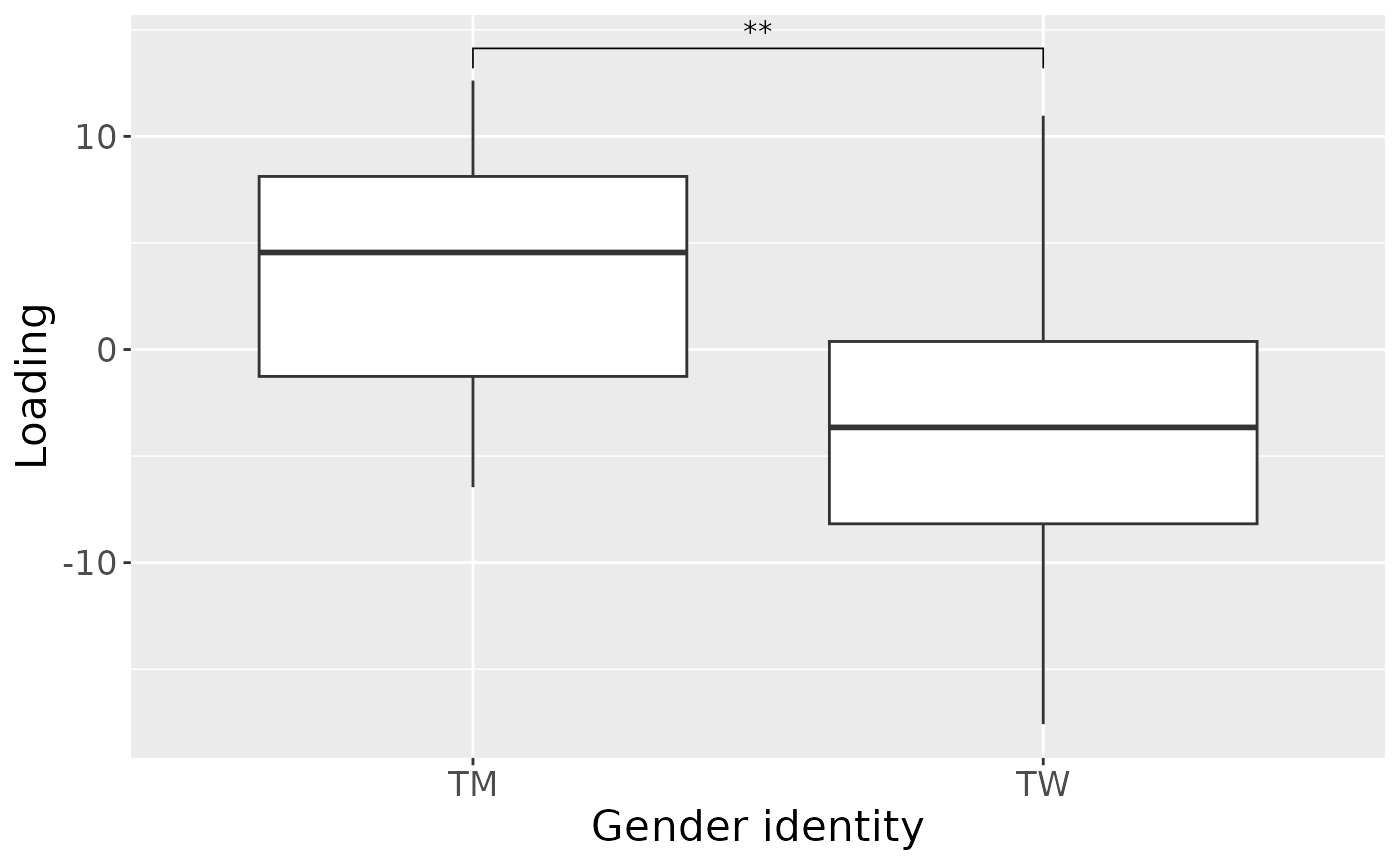
b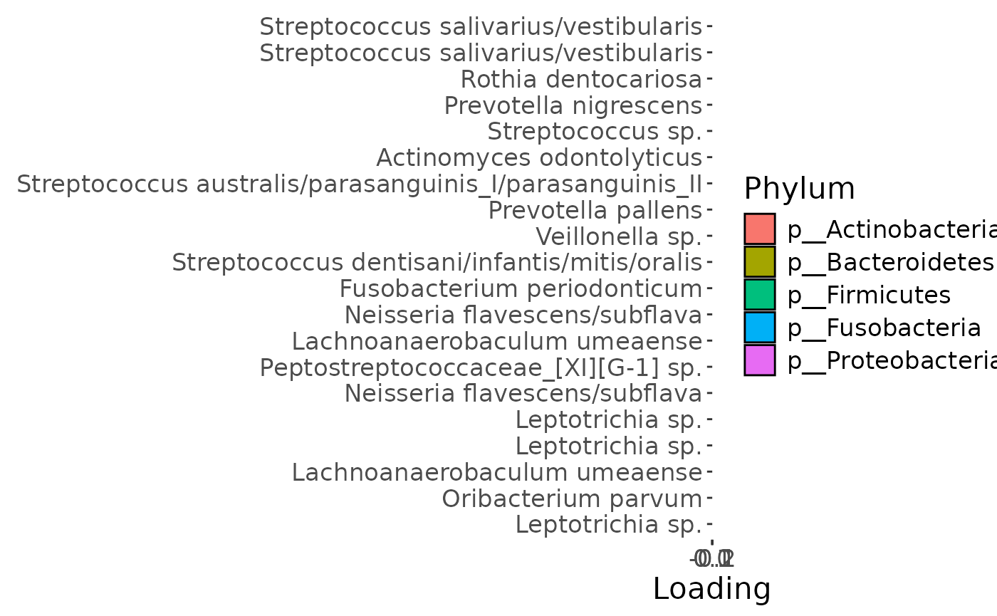
c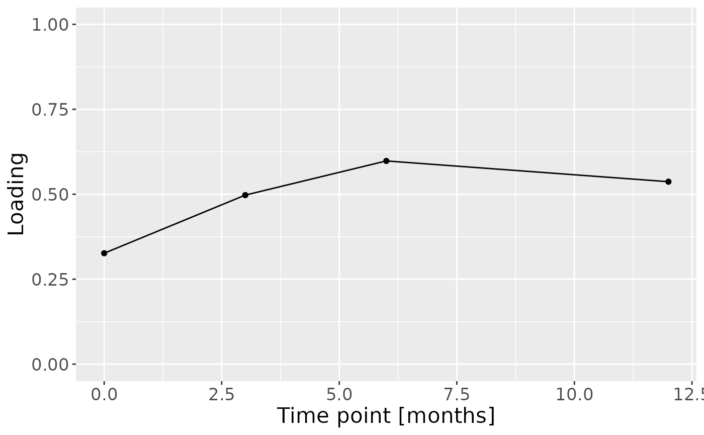
Positively loaded microbiota including Streptococcus salivarius / vestibularis, Rothia dentocariosa, Prevotella nigrescens, Streptococcus sp., Actinomyces odontolyticus, Streptococcus australis / parasanguinis, Prevotella pallens, Veillonella sp., and Streptococcus dentisani / infantis / mitis / oralis were enriched in transfeminine participants and depleted in transmasculine participants. Conversely, negatively loaded microbiota including Leptotrichia spp., Oribacterium parvum, Neisseria flavescens / subflava, Peptostreptococcaceae sp., Lachnoanaerobaculum umeaense, and Fusobacterium periodonticum were enriched in transmasculine participants and depleted in transfeminine participants. The time mode loadings indicate that inter-subject differences due to GAHT increased over time, and reached a maximum at month six.
Salivary microbiome
NPLS was next applied to supervise the decomposition using the difference in free testosterone between baseline and month three of GAHT as the dependent variable (y). The model selection procedure revealed that a one-component NPLS model corresponded to the RMSECV minimum, explaining 4.8% of the variation in X, and 33.1% of the variation in y. The commented code below performs the procedure, and is not rerun here due to computational limitations.
# CV_saliva = NPLStoolbox::ncrossreg(processedSaliva$data, Ynorm_saliva, maxNumComponents = 10)
# a=CV_saliva$varExp %>% pivot_longer(-numComponents) %>% ggplot(aes(x=as.factor(numComponents),y=value,col=as.factor(name),group=as.factor(name))) + geom_line() + geom_point() + xlab("Number of components") + ylab("Variance explained (%)") + theme(legend.position="none")
# b=CV_saliva$RMSE %>% ggplot(aes(x=numComponents,y=RMSE)) + geom_line() + geom_point() + xlab("Number of components") + ylab("RMSECV")
# ggarrange(a,b) # 1
# npls_saliva = NPLStoolbox::triPLS1(processedSaliva$data, Ynorm_saliva, 1)
npls_saliva = readRDS("./GOHTRANS/NPLS_saliva_deltaT.RDS")

npls_saliva$varExpX
#> [1] 4.786039
npls_saliva$varExpY
#> [1] 33.14521
As expected, MLR analysis revealed that the model captured variation exclusively associated with gender identity.
testMetadata(npls_saliva, 1, processedSaliva)
#> Joining with `by = join_by(subject, GenderID)`
#>       Term     Estimate                                        CI    P_value
#> 1 GenderID -151.2510652  -0.279791282367381 – -0.0227108480443339 0.02294631
#> 2      Age    3.0405540  -0.0113505594011473 – 0.0174316674214563 0.66719488
#> 3      BOP    5.3079802 -0.00314350146723959 – 0.0137594618286484 0.20766265
#> 4     CODS   -3.7471649  -0.0181342709520459 – 0.0106399411508536 0.59641461
#> 5       XI   -0.1190497  -0.0150050109726752 – 0.0147669115500696 0.98698934
#>    P_adjust
#> 1 0.1147315
#> 2 0.8339936
#> 3 0.5191566
#> 4 0.8339936
#> 5 0.9869893
a = processedSaliva$mode1 %>%
  mutate(comp=npls_saliva$Fac[[1]][,1]) %>%
  ggplot(aes(x=as.factor(GenderID),y=comp)) +
  geom_boxplot() +
  stat_compare_means(comparisons=list(c("TM","TW")), label="p.signif") +
  xlab("Gender identity") +
  ylab("Loading") +
  theme(text=element_text(size=16))

temp = processedSaliva$mode2 %>%
  as_tibble() %>%
  mutate(Component_1 = -1*npls_saliva$Fac[[2]][,1]) %>%
  mutate(Genus = gsub("g__", "", Genus), Species = gsub("s__", "", Species)) %>%
  mutate(Species = gsub("\\(", "", Species)) %>%
  mutate(Species = gsub("\\)", "", Species))

fixedSpeciesNames = str_split_fixed(temp$Species, "/", 5) %>%
  as_tibble() %>%
  mutate(dplyr::across(.cols = everything(), .fns = ~ dplyr::if_else(stringr::str_detect(.x, "sp."), "", .x)))
fixedSpeciesNames[fixedSpeciesNames$V1 == "", "V1"] = "sp."
fixedSpeciesNames = fixedSpeciesNames %>%
  mutate(name=paste0(V1, "/", V2)) %>%
  mutate(name=gsub("/$", "", name)) %>%
  mutate(name=paste0(name, "/", V3)) %>%
  mutate(name=gsub("/$", "", name)) %>%
  mutate(name=paste0(name, "/", V4)) %>%
  mutate(name=gsub("/$", "", name)) %>%
  mutate(name=paste0(name, "/", V5)) %>%
  mutate(name=gsub("/$", "", name))

temp$Species = fixedSpeciesNames$name
temp$name = paste0(temp$Genus, " ", temp$Species)
temp[temp$name == " sp.", "name"] = "Unclassified"
temp[temp$name == " ", "name"] = "Unclassified"
temp[temp$name == " sp.", "name"] = "Unclassified"

temp = temp %>%
  arrange(Component_1) %>%
  mutate(index=1:nrow(.)) %>%
  filter(index %in% c(1:10,251:260))

b=temp %>%
  ggplot(aes(x=Component_1,y=as.factor(index),fill=as.factor(Phylum))) +
  geom_bar(stat="identity", col="black") +
  scale_y_discrete(label=temp$name) +
  xlab("Loading") +
  ylab("") +
  guides(fill=guide_legend(title="Phylum")) +
  theme(text=element_text(size=16))

c = npls_saliva$Fac[[3]][,1] %>%
  as_tibble() %>%
  mutate(value=value) %>%
  mutate(timepoint=c(0,3,6,12)) %>%
  ggplot(aes(x=timepoint,y=value)) +
  geom_line() +
  geom_point() +
  xlab("Time point [months]") +
  ylab("Loading") +
  ylim(0,1)

a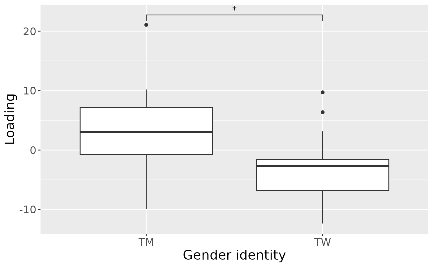
b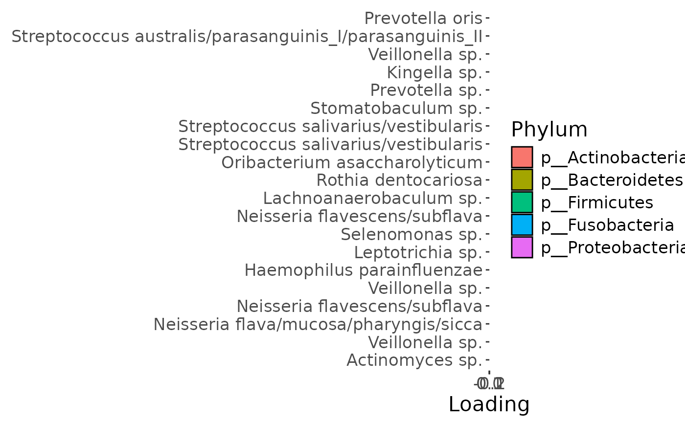
c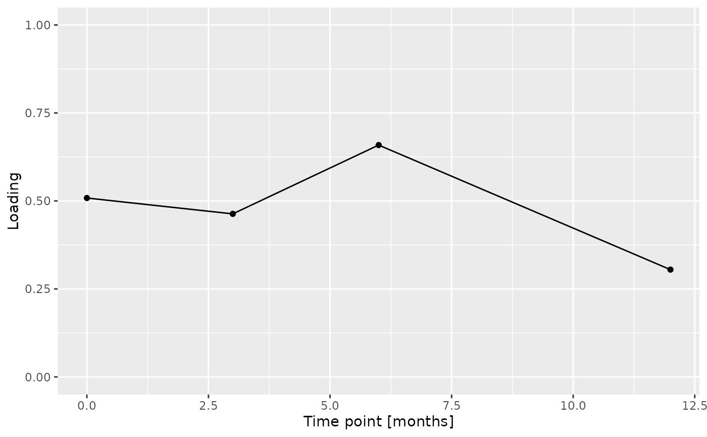
Positively loaded microbiota including Prevotella oris, Streptococcus australis / parasanguinis, Veillonella sp., Kingella sp., Prevotella sp., Stomatobaculum sp., Streptococcus salivarius / vestibularis, Oribacterium asaccharolyticum, and Rothia dentocariosa were enriched in transfeminine participants and depleted in transmasculine participants. Conversely, negatively loaded microbiota including Actinomyces sp., Veillonella spp., Neisseria flava / mucosa / pharyngis / sicca, Neisseria flavescens / subflava, Haemophilus parainfluenzae, Leptotrichia sp., Selenomonas sp., and Lachnoanaerobaculum sp. were enriched in transmasculine participants and depleted in transfeminine participants. The time mode loadings indicate that inter-subject differences due to GAHT reach a maximum at month six, before dropping sharply.
Salivary cytokines
NPLS was next applied to supervise the decomposition using the difference in free testosterone between baseline and month three of GAHT as the dependent variable (y). The model selection procedure revealed that a two-component NPLS model corresponded to the RMSECV minimum, but was biologically uninterpretable. Therefore a one-component NPLS model was selected, explaining 48.9% of the variation in X, and 34.7% of the variation in y. The commented code below performs the procedure, and is not rerun here due to computational limitations.
# CV_cyto = NPLStoolbox::ncrossreg(processedCytokines$data, Ynorm_cytokine, maxNumComponents = 10)
# a=CV_cyto$varExp %>% pivot_longer(-numComponents) %>% ggplot(aes(x=as.factor(numComponents),y=value,col=as.factor(name),group=as.factor(name))) + geom_line() + geom_point() + xlab("Number of components") + ylab("Variance explained (%)") + theme(legend.position="none")
# b=CV_cyto$RMSE %>% ggplot(aes(x=numComponents,y=RMSE)) + geom_line() + geom_point() + xlab("Number of components") + ylab("RMSECV")
# ggarrange(a,b) # 1
# npls_cyto = NPLStoolbox::triPLS1(processedCytokines$data, Ynorm_cytokine, 1)
npls_cyto = readRDS("./GOHTRANS/NPLS_cyto_deltaT.RDS")

npls_cyto$varExpX
#> [1] 27.12405
npls_cyto$varExpY
#> [1] 21.17445
Unexpectedly, MLR analysis revealed that the model captured uninterpretable variation.
testMetadata(npls_cyto, 1, processedCytokines)
#> Joining with `by = join_by(subject, GenderID)`
#>       Term    Estimate                                        CI    P_value
#> 1 GenderID -157.807812   -0.373026599093144 – 0.0574109754715683 0.13812064
#> 2      Age    7.156904  -0.0162848911715474 – 0.0305986991843004 0.52320055
#> 3      BOP   15.067426 -0.00127830792711726 – 0.0314131605144182 0.06807157
#> 4     CODS  -51.616492    -0.402993987873639 – 0.299761004737455 0.75736016
#> 5       XI    8.824141  -0.0164756264949713 – 0.0341239080914935 0.46680152
#>    P_adjust
#> 1 0.3453016
#> 2 0.6540007
#> 3 0.3403578
#> 4 0.7573602
#> 5 0.6540007
Salivary biochemistry
NPLS was next applied to the salivary biochemistry data block to supervise the decomposition using the difference in free testosterone between baseline and month three of GAHT as the dependent variable (y). The model selection procedure revealed that a two-component NPLS model corresponded to the RMSECV minimum, but was biologically uninterpretable. Therefore, a one-component NPLS model was selected, explaining 16.4% of the variation in X, and 25.3% of the variation in y.
# CV_bio = NPLStoolbox::ncrossreg(processedBiochemistry$data, Ynorm_biochem, maxNumComponents=10)
# a=CV_bio$varExp %>% pivot_longer(-numComponents) %>% ggplot(aes(x=as.factor(numComponents),y=value,col=as.factor(name),group=as.factor(name))) + geom_line() + geom_point() + xlab("Number of components") + ylab("Variance explained (%)") + theme(legend.position="none")
# b=CV_bio$RMSE %>% ggplot(aes(x=numComponents,y=RMSE)) + geom_line() + geom_point() + xlab("Number of components") + ylab("RMSECV")
# ggarrange(a,b) # 1
# npls_bio = NPLStoolbox::triPLS1(processedBiochemistry$data, Ynorm_biochem, 1)
npls_bio = readRDS("./GOHTRANS/NPLS_bio_deltaT.RDS")

npls_bio$varExpX
#> [1] 16.41914
npls_bio$varExpY
#> [1] 25.30623
As expected, MLR analysis revealed that the model captured variation exclusively associated with gender identity.
testMetadata(npls_bio, 1, processedBiochemistry)
#> Joining with `by = join_by(subject, GenderID)`
#>       Term    Estimate                                        CI    P_value
#> 1 GenderID -156.225906  -0.285656710827189 – -0.0267951010155874 0.01996409
#> 2      Age   -4.528260 -0.0190190823798637 – 0.00996256139587153 0.52570273
#> 3      BOP   -1.854863 -0.0103649001380471 – 0.00665517492477034 0.65737051
#> 4     CODS    2.516212   -0.0119705747472031 – 0.017002998779039 0.72355422
#> 5       XI    3.968734  -0.0110203642172829 – 0.0189578323409959 0.59037036
#>     P_adjust
#> 1 0.09982045
#> 2 0.72355422
#> 3 0.72355422
#> 4 0.72355422
#> 5 0.72355422
a = processedBiochemistry$mode1 %>%
  mutate(comp=npls_bio$Fac[[1]][,1]) %>%
  ggplot(aes(x=as.factor(GenderID),y=comp)) +
  geom_boxplot() +
  stat_compare_means(comparisons=list(c("TM","TW")), label="p.signif") +
  xlab("Gender identity") +
  ylab("Loading") +
  theme(text=element_text(size=16))

temp = processedBiochemistry$mode2 %>%
  mutate(Comp = -1*npls_bio$Fac[[2]][,1]) %>%
  arrange(Comp) %>%
  mutate(index=1:nrow(.)) %>%
  mutate(V1 = c("pH", "S-IgA", "Chitinase", "MUC-5B", "Amylase", "Total protein", "Lysozyme"))

b = temp %>%
  ggplot(aes(x=Comp,y=as.factor(index))) +
  geom_bar(stat="identity", col="black") +
  xlab("Loading") +
  ylab("") +
  scale_y_discrete(labels=temp$V1) +
  theme(text=element_text(size=16))

c = npls_bio$Fac[[3]][,1] %>%
  as_tibble() %>%
  mutate(value=value) %>%
  mutate(timepoint=c(0,3,6,12)) %>%
  ggplot(aes(x=timepoint,y=value)) +
  geom_line() +
  geom_point() +
  xlab("Time point [months]") +
  ylab("Loading") +
  ylim(0,1) +
  theme(text=element_text(size=16))

a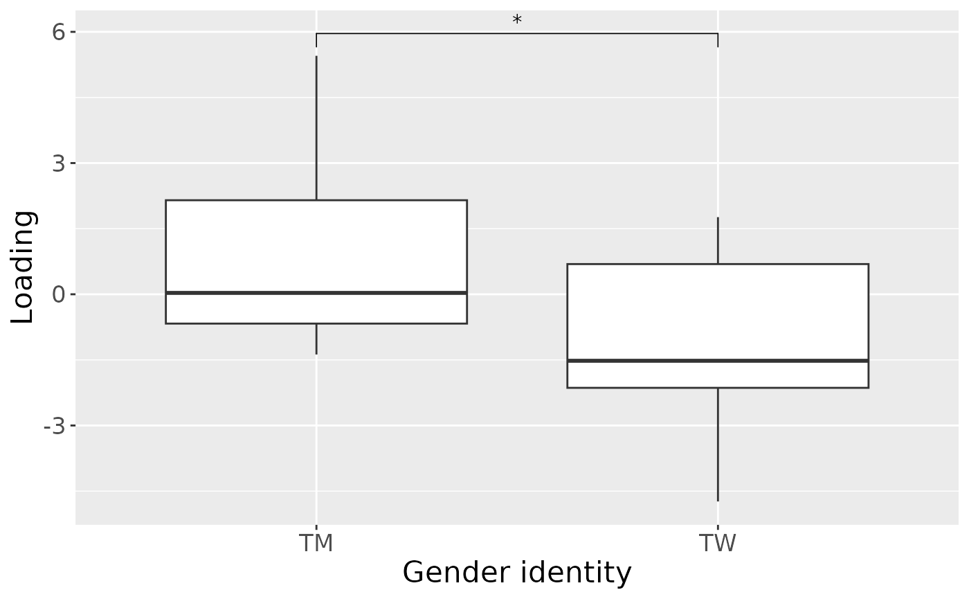
b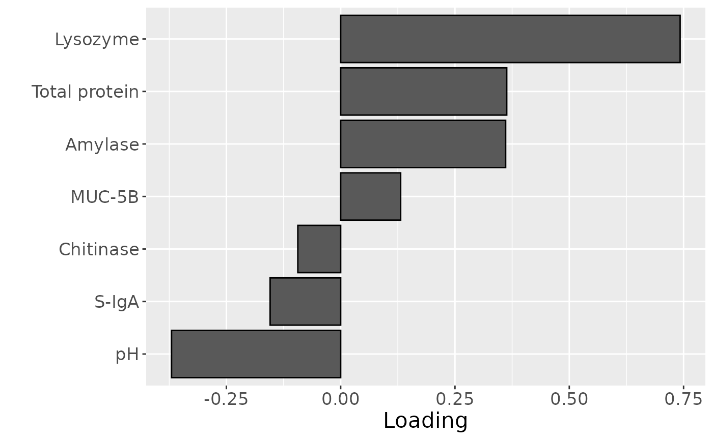
c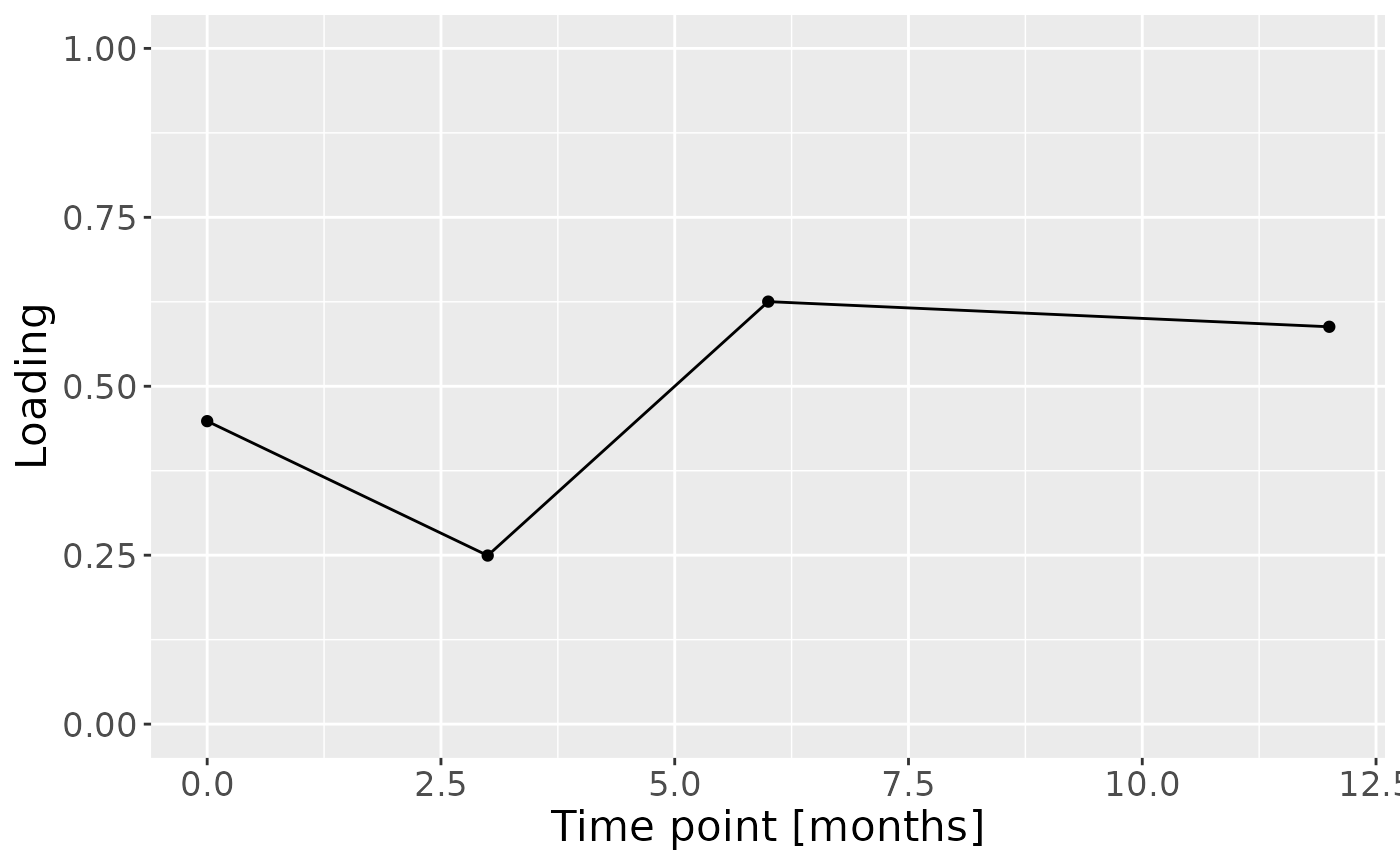
Positively loaded features including lysozyme, total protein, amylase, and MUC-5B had higher levels in transfeminine participants and lower levels in transmasculine participants. Conversely, negatively loaded features including pH, S-IgA, and chitinase had higher levels in transmasculine participants and lower levels in transfeminine participants. The time mode loadings indicate that these differences mainly occurred after the six-month mark of GAHT.