TIFN2: Red fluorescent plaque development in gingivitis
2025-08-31
Source:vignettes/articles/TIFN2.Rmd
TIFN2.RmdIntroduction
This article presents the NPLS results of the TIFN2 dataset discussed in Chapter 4 of my dissertation.
Preamble
library(dplyr)
#>
#> Attaching package: 'dplyr'
#> The following objects are masked from 'package:stats':
#>
#>     filter, lag
#> The following objects are masked from 'package:base':
#>
#>     intersect, setdiff, setequal, union
library(tidyr)
library(parafac4microbiome)
library(NPLStoolbox)
library(CMTFtoolbox)
#>
#> Attaching package: 'CMTFtoolbox'
#> The following object is masked from 'package:NPLStoolbox':
#>
#>     npred
#> The following objects are masked from 'package:parafac4microbiome':
#>
#>     fac_to_vect, reinflateFac, reinflateTensor, vect_to_fac
library(ggplot2)
library(ggpubr)
library(scales)
library(ggpattern)
rf_data = read.csv("./TIFN2/RFdata.csv")
colnames(rf_data) = c("subject", "id", "fotonr", "day", "group", "RFgroup", "MQH", "SPS(tm)", "Area_delta_R30", "Area_delta_Rmax", "Area_delta_R30_x_Rmax", "gingiva_mean_R_over_G", "gingiva_mean_R_over_G_upper_jaw", "gingiva_mean_R_over_G_lower_jaw")
rf_data = rf_data %>% as_tibble()

rf_data[rf_data$subject == "VSTPHZ", 1] = "VSTPH2"
rf_data[rf_data$subject == "D2VZH0", 1] = "DZVZH0"
rf_data[rf_data$subject == "DLODNN", 1] = "DLODDN"
rf_data[rf_data$subject == "O3VQFX", 1] = "O3VQFQ"
rf_data[rf_data$subject == "F80LGT", 1] = "F80LGF"
rf_data[rf_data$subject == "26QQR0", 1] = "26QQrO"

rf_data2 = read.csv("./TIFN2/red_fluorescence_data.csv") %>% as_tibble()
rf_data2 = rf_data2[,c(2,4,181:192)]
rf_data = rf_data %>% left_join(rf_data2)
#> Joining with `by = join_by(id, day)`

rf = rf_data %>% select(subject, RFgroup) %>% unique()
age_gender = read.csv("./TIFN2/Ploeg_subjectMetadata.csv", sep=";")
age_gender = age_gender[2:nrow(age_gender),2:ncol(age_gender)]
age_gender = age_gender %>% as_tibble() %>% filter(onderzoeksgroep == 0) %>% select(naam, leeftijd, geslacht)
colnames(age_gender) = c("subject", "age", "gender")

# Correction for incorrect subject ids
age_gender[age_gender$subject == "VSTPHZ", 1] = "VSTPH2"
age_gender[age_gender$subject == "D2VZH0", 1] = "DZVZH0"
age_gender[age_gender$subject == "DLODNN", 1] = "DLODDN"
age_gender[age_gender$subject == "O3VQFX", 1] = "O3VQFQ"
age_gender[age_gender$subject == "F80LGT", 1] = "F80LGF"
age_gender[age_gender$subject == "26QQR0", 1] = "26QQrO"

age_gender = age_gender %>% arrange(subject)
mapping = c(-14,0,2,5,9,14,21)

testMetadata = function(model, comp, metadata){
  transformedSubjectLoadings = transformPARAFACloadings(model$Fac, 1)[,comp]
  transformedSubjectLoadings = transformedSubjectLoadings / norm(transformedSubjectLoadings, "2")

  metadata = metadata$mode1 %>% left_join(vanderPloeg2024$red_fluorescence %>% select(subject,day,Area_delta_R30,plaquepercent,bomppercent) %>% filter(day==14), by="subject")

  result = lm(transformedSubjectLoadings ~ plaquepercent + bomppercent + Area_delta_R30 + gender + age, data=metadata)

  # Extract coefficients and confidence intervals
  coef_estimates <- summary(result)$coefficients
  conf_intervals <- confint(result)

  # Remove intercept
  coef_estimates <- coef_estimates[rownames(coef_estimates) != "(Intercept)", ]
  conf_intervals <- conf_intervals[rownames(conf_intervals) != "(Intercept)", ]

  # Combine into a clean data frame
  summary_table <- data.frame(
    Term     = rownames(coef_estimates),
    Estimate = coef_estimates[, "Estimate"] * 1e3,
    CI       = paste0(
                 conf_intervals[, 1], " – ",
                 conf_intervals[, 2]
               ),
    P_value  = coef_estimates[, "Pr(>|t|)"],
    P_adjust = p.adjust(coef_estimates[, "Pr(>|t|)"], "BH"),
    row.names = NULL
  )

  return(summary_table)
}

testFeatures = function(model, metadata, componentNum, metadataVar){
  df = metadata$mode1 %>% left_join(rf_data %>% filter(day==14)) %>% left_join(age_gender)
  topIndices = metadata$mode2 %>% mutate(index=1:nrow(.), Comp = model$Fac[[2]][,componentNum]) %>% arrange(desc(Comp)) %>% head() %>% select(index) %>% pull()
  bottomIndices = metadata$mode2 %>% mutate(index=1:nrow(.), Comp = model$Fac[[2]][,componentNum]) %>% arrange(desc(Comp)) %>% tail() %>% select(index) %>% pull()

  timepoint = which(abs(model$Fac[[3]][,componentNum]) == max(abs(model$Fac[[3]][,componentNum])))

  Xhat = parafac4microbiome::reinflateTensor(model$Fac[[1]][,componentNum], model$Fac[[2]][,componentNum], model$Fac[[3]][,componentNum])
  y = df[metadataVar]

  print("Positive loadings:")
  print(cor(Xhat[,topIndices[1],timepoint], y))
  print("Negative loadings:")
  print(cor(Xhat[,bottomIndices[1],timepoint], y))
}

plotFeatures = function(mode2, model, componentNum, flip=FALSE){

  if(flip==TRUE){
    df = mode2 %>% mutate(Comp = -1*model$Fac[[2]][,componentNum]) %>% arrange(Comp) %>% filter(Species != "") %>% mutate(index=1:nrow(.), name = paste(Genus, Species))
  } else{
    df = mode2 %>% mutate(Comp = model$Fac[[2]][,componentNum]) %>% arrange(Comp) %>% filter(Species != "") %>% mutate(index=1:nrow(.), name = paste(Genus, Species))
  }
  df = rbind(df %>% head(n=10), df %>% tail(n=10))

  plot=df %>%
    ggplot(aes(x=Comp,y=as.factor(index),fill=as.factor(Phylum))) +
    geom_bar(stat="identity", col="black") +
    scale_y_discrete(label=df$name) +
    xlab("Loading") +
    ylab("") +
    guides(fill=guide_legend(title="Phylum")) +
    theme(text=element_text(size=16))

  return(plot)
}
phylum_colors = hue_pal()(7)
processedTongue = processDataCube(parafac4microbiome::vanderPloeg2024$tongue, sparsityThreshold=0.50, considerGroups=TRUE, groupVariable="RFgroup", CLR=TRUE, centerMode=1, scaleMode=2)
processedLowling = processDataCube(parafac4microbiome::vanderPloeg2024$lower_jaw_lingual, sparsityThreshold=0.50, considerGroups=TRUE, groupVariable="RFgroup", CLR=TRUE, centerMode=1, scaleMode=2)
processedLowinter = processDataCube(parafac4microbiome::vanderPloeg2024$lower_jaw_interproximal, sparsityThreshold=0.50, considerGroups=TRUE, groupVariable="RFgroup", CLR=TRUE, centerMode=1, scaleMode=2)
processedUpling = processDataCube(parafac4microbiome::vanderPloeg2024$upper_jaw_lingual, sparsityThreshold=0.50, considerGroups=TRUE, groupVariable="RFgroup", CLR=TRUE, centerMode=1, scaleMode=2)
processedUpinter = processDataCube(parafac4microbiome::vanderPloeg2024$upper_jaw_interproximal, sparsityThreshold=0.50, considerGroups=TRUE, groupVariable="RFgroup", CLR=TRUE, centerMode=1, scaleMode=2)
processedSaliva = processDataCube(parafac4microbiome::vanderPloeg2024$saliva, sparsityThreshold=0.50, considerGroups=TRUE, groupVariable="RFgroup", CLR=TRUE, centerMode=1, scaleMode=2)
processedMetabolomics = parafac4microbiome::vanderPloeg2024$metabolomics
Y = processedTongue$mode1 %>% left_join(vanderPloeg2024$red_fluorescence %>% select(subject,Area_delta_R30,day) %>% filter(day==14)) %>% select(Area_delta_R30) %>% pull()
#> Joining with `by = join_by(subject)`
Ycnt = Y - mean(Y)

Ymetab = processedMetabolomics$mode1 %>% left_join(vanderPloeg2024$red_fluorescenc %>% select(subject,Area_delta_R30,day) %>% filter(day==14)) %>% select(Area_delta_R30) %>% pull()
#> Joining with `by = join_by(subject)`
Ymetab_cnt = Ymetab - mean(Ymetab)
Tongue microbiome
NPLS was subsequently applied to supervise the decomposition using the percentage of sites that were covered in red fluorescent plaque (RF%) as dependent variable (y). The model selection procedure revealed that three components were appropriate due to the observation of an elbow in the variance explained for X, explaining 31.3% of variation in X and 71.7% of variation in y. The commented code below performs the procedure, and is not rerun here due to computational limitations.
# CV_tongue = NPLStoolbox::ncrossreg(processedTongue$data, Ycnt, maxNumComponents = 10)
# a=CV_tongue$varExp %>% pivot_longer(-numComponents) %>% ggplot(aes(x=as.factor(numComponents),y=value,col=as.factor(name),group=as.factor(name))) + geom_line() + geom_point() + xlab("Number of components") + ylab("Variance explained (%)") + theme(legend.position="none")
# b=CV_tongue$RMSE %>% ggplot(aes(x=as.factor(numComponents),y=RMSE,group=1)) + geom_line() + geom_point() + xlab("Number of components") + ylab("RMSECV")
# ggarrange(a,b)
# npls_tongue = NPLStoolbox::triPLS1(processedTongue$data, Ycnt, 3)
npls_tongue = readRDS("./TIFN2/NPLS_tongue.RDS")

npls_tongue$varExpX
#> [1] 31.32394
npls_tongue$varExpY
#> [1] 71.68906
As expected, the first NPLS component captured variation exclusively associated with RF%, while the second component captured variation exclusively associated with subject age, and the third component captured variation associated with plaque% and subject age.
testMetadata(npls_tongue, 1, processedTongue)
#>             Term  Estimate                                         CI
#> 1  plaquepercent -1.474762 -0.00708656930332159 – 0.00413704497828965
#> 2    bomppercent  1.631592  -0.0018744665656207 – 0.00513764997731347
#> 3 Area_delta_R30 11.077971   0.00400772030295017 – 0.0181482211785528
#> 4         gender 36.330007        -0.063223285837 – 0.135883300205861
#> 5            age  3.166008  -0.00570115787648339 – 0.0120331734187125
#>       P_value   P_adjust
#> 1 0.597056195 0.59705619
#> 2 0.351269153 0.59170540
#> 3 0.003072009 0.01536005
#> 4 0.463727425 0.59170540
#> 5 0.473364318 0.59170540
testMetadata(npls_tongue, 2, processedTongue)
#>             Term   Estimate                                          CI
#> 1  plaquepercent   5.382195  -0.000686132570085629 – 0.0114505233390118
#> 2    bomppercent  -1.872716  -0.00566399213852543 – 0.00191856046358201
#> 3 Area_delta_R30   1.020862   -0.00662455365668888 – 0.0086662777282295
#> 4         gender -21.544052     -0.129196011019746 – 0.0861079065423951
#> 5            age -10.473955 -0.0200624648453823 – -0.000885444742297401
#>      P_value  P_adjust
#> 1 0.08039408 0.2009852
#> 2 0.32284992 0.5380832
#> 3 0.78792781 0.7879278
#> 4 0.68701099 0.7879278
#> 5 0.03317110 0.1658555
testMetadata(npls_tongue, 3, processedTongue)
#>             Term    Estimate                                         CI
#> 1  plaquepercent  -7.5520385 -0.0125229141152452 – -0.00258116287242108
#> 2    bomppercent  -0.7879148 -0.00389354174770562 – 0.00231771218586553
#> 3 Area_delta_R30  -0.2122868 -0.00647503505852898 – 0.00605046150851769
#> 4         gender -29.3520691    -0.117535255934982 – 0.0588311176394589
#> 5            age  15.5190376   0.00766460204790137 – 0.0233734731629338
#>        P_value    P_adjust
#> 1 0.0039690081 0.009922520
#> 2 0.6097561177 0.762195147
#> 3 0.9455292860 0.945529286
#> 4 0.5036538142 0.762195147
#> 5 0.0003022874 0.001511437
testFeatures(npls_tongue, processedTongue, 1, "Area_delta_R30") # flip
#> Joining with `by = join_by(subject, RFgroup)`
#> Joining with `by = join_by(subject, age, gender)`
#> [1] "Positive loadings:"
#>      Area_delta_R30
#> [1,]     -0.5331209
#> [1] "Negative loadings:"
#>      Area_delta_R30
#> [1,]      0.5331209

a = processedTongue$mode1 %>%
  mutate(Component_1 = npls_tongue$Fac[[1]][,1]) %>%
  left_join(rf_data %>% select(subject,day,Area_delta_R30,plaquepercent,bomppercent) %>% filter(day==14), by="subject") %>%
  ggplot(aes(x=Area_delta_R30,y=Component_1)) +
  geom_point() +
  xlab("RF%") +
  ylab("Loading") +
  stat_cor() +
  theme(text=element_text(size=16))

b = plotFeatures(processedTongue$mode2, npls_tongue, 1, flip=TRUE) + scale_fill_manual(values=phylum_colors[-c(3,7)]) + theme(legend.position="none")

c = processedTongue$mode3 %>%
  mutate(Component_1 = -1*npls_tongue$Fac[[3]][,1], day=c(-14,0,2,5,9,14,21)) %>%
  ggplot(aes(x=day,y=Component_1)) +
  annotate(geom = "rect", xmin = 0, xmax = 14, ymin = -Inf, ymax = Inf, fill = "red", colour = "black", alpha=0.25) +
  geom_line() +
  geom_point() +
  xlab("Time point [days]") +
  ylab("Loading") +
  ylim(0,1) +
  theme(legend.position="none", text=element_text(size=16))

a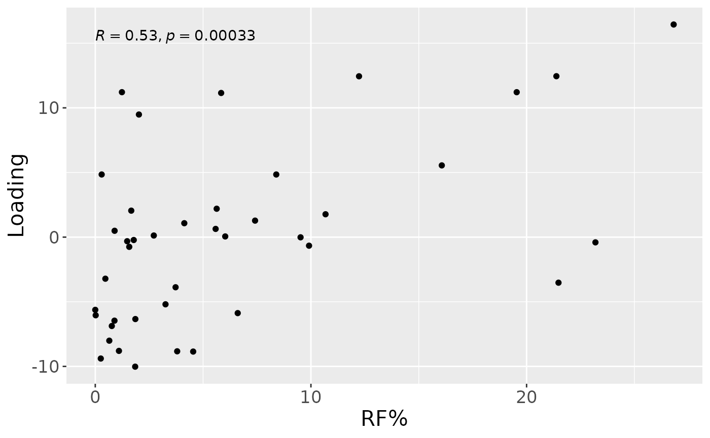
b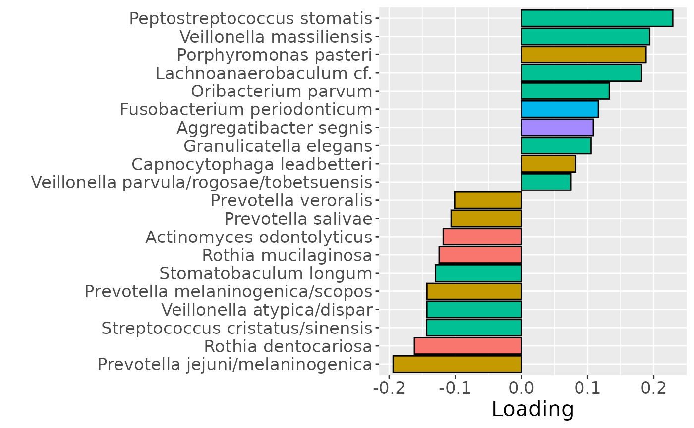
c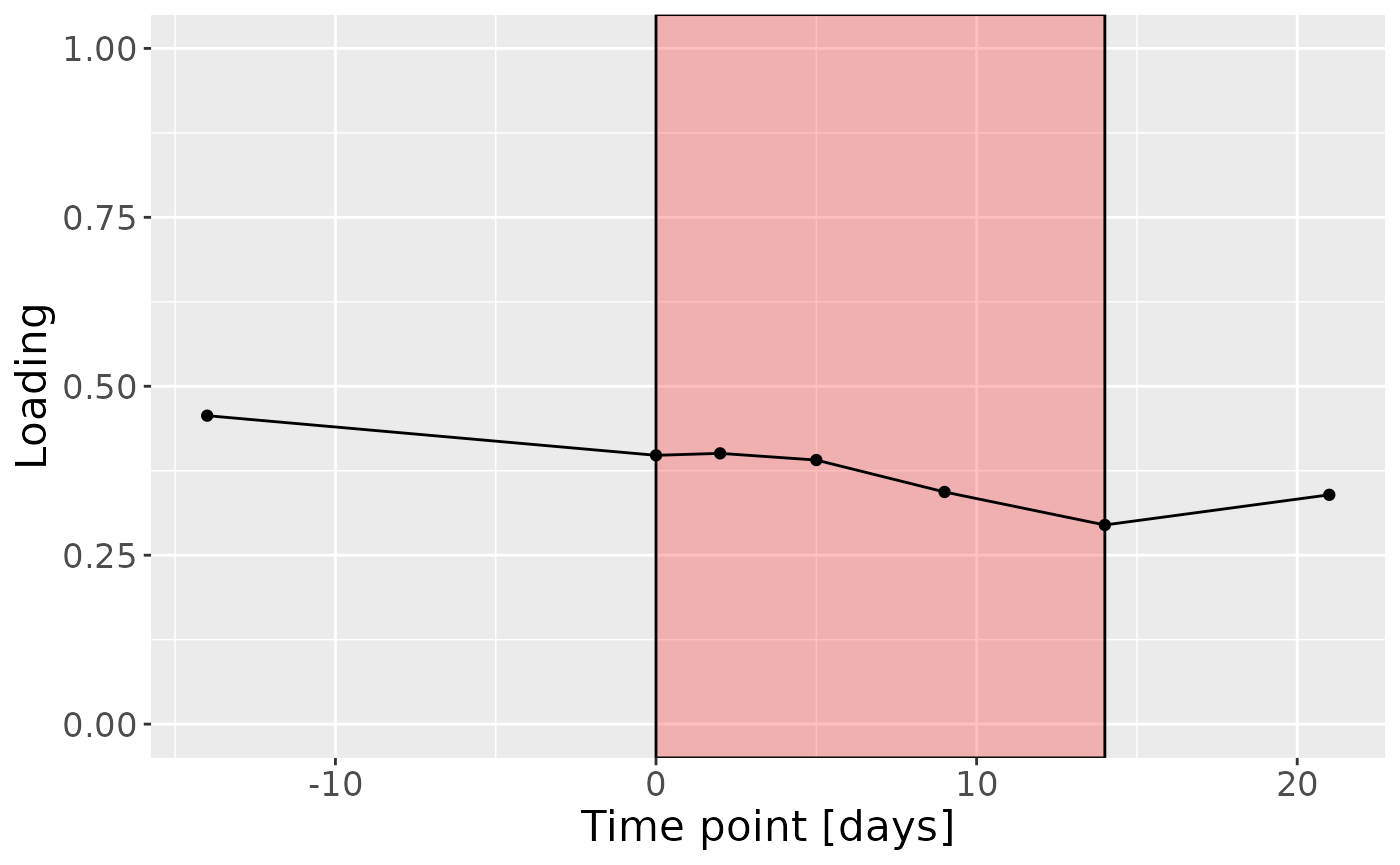
testFeatures(npls_tongue, processedTongue, 2, "age") # flip
#> Joining with `by = join_by(subject, RFgroup)`
#> Joining with `by = join_by(subject, age, gender)`
#> [1] "Positive loadings:"
#>             age
#> [1,] -0.2936364
#> [1] "Negative loadings:"
#>            age
#> [1,] 0.2936364

a = processedTongue$mode1 %>%
  mutate(Component_1 = npls_tongue$Fac[[1]][,2]) %>%
  left_join(rf_data %>% select(subject,day,Area_delta_R30,plaquepercent,bomppercent) %>% filter(day==14), by="subject") %>%
  ggplot(aes(x=age,y=Component_1)) +
  geom_point() +
  xlab("Age") +
  ylab("Loading") +
  stat_cor() +
  theme(text=element_text(size=16))

b = plotFeatures(processedTongue$mode2, npls_tongue, 2, flip=TRUE) + scale_fill_manual(values=phylum_colors[-c(6,7)]) + theme(legend.position="none")

c = processedTongue$mode3 %>%
  mutate(Component_1 = npls_tongue$Fac[[3]][,2], day=c(-14,0,2,5,9,14,21)) %>%
  ggplot(aes(x=day,y=Component_1)) +
  annotate(geom = "rect", xmin = 0, xmax = 14, ymin = -Inf, ymax = Inf, fill = "red", colour = "black", alpha=0.25) +
  geom_line() +
  geom_point() +
  xlab("Time point [days]") +
  ylab("Loading") +
  ylim(0,1) +
  theme(legend.position="none", text=element_text(size=16))

a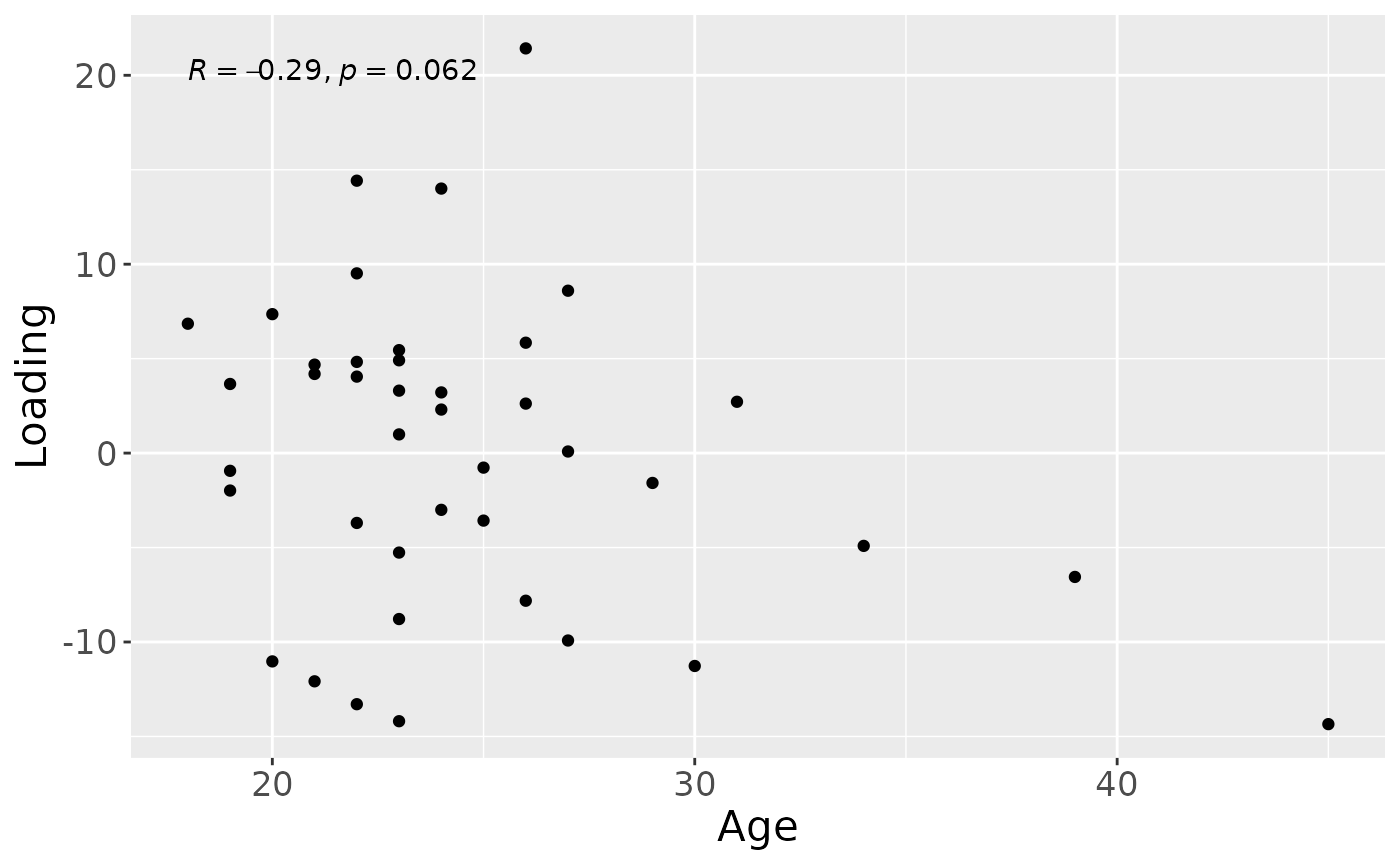
b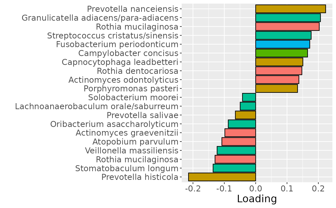
c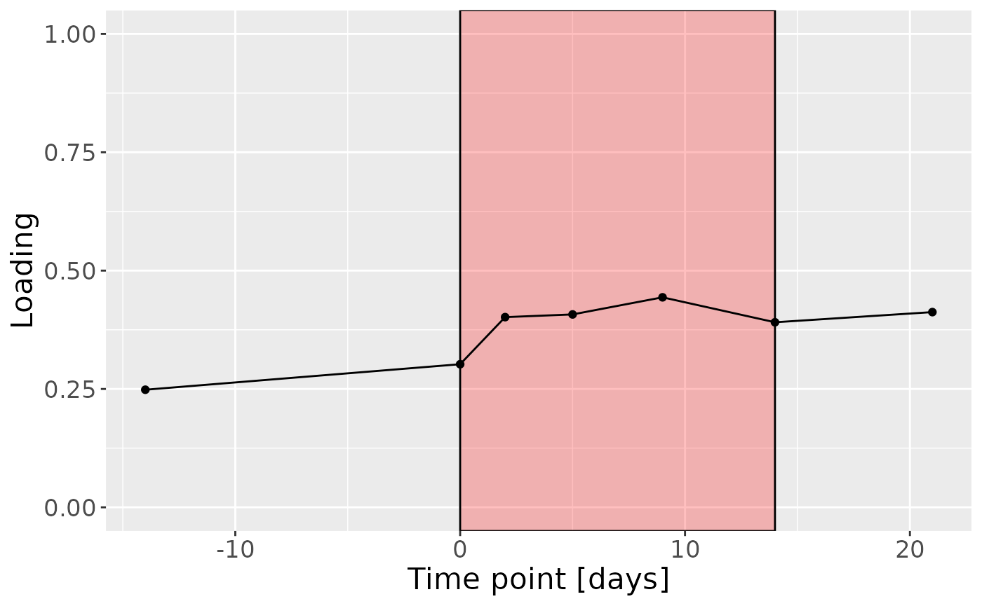
testFeatures(npls_tongue, processedTongue, 3, "age") # flip
#> Joining with `by = join_by(subject, RFgroup)`
#> Joining with `by = join_by(subject, age, gender)`
#> [1] "Positive loadings:"
#>             age
#> [1,] -0.5022835
#> [1] "Negative loadings:"
#>            age
#> [1,] 0.5022835
testFeatures(npls_tongue, processedTongue, 3, "plaquepercent") # flip
#> Joining with `by = join_by(subject, RFgroup)`
#> Joining with `by = join_by(subject, age, gender)`
#> [1] "Positive loadings:"
#>      plaquepercent
#> [1,]     0.4065813
#> [1] "Negative loadings:"
#>      plaquepercent
#> [1,]    -0.4065813

a = processedTongue$mode1 %>%
  mutate(Component_1 = npls_tongue$Fac[[1]][,3]) %>%
  left_join(rf_data %>% select(subject,day,Area_delta_R30,plaquepercent,bomppercent) %>% filter(day==14), by="subject") %>%
  ggplot(aes(x=age,y=Component_1)) +
  geom_point() +
  xlab("Age") +
  ylab("Loading") +
  stat_cor() +
  theme(text=element_text(size=16))

b = plotFeatures(processedTongue$mode2, npls_tongue, 3, flip=TRUE) + scale_fill_manual(values=phylum_colors[-c(3,7)]) + theme(legend.position="none")

c = processedTongue$mode3 %>%
  mutate(Component_1 = -1*npls_tongue$Fac[[3]][,3], day=c(-14,0,2,5,9,14,21)) %>%
  ggplot(aes(x=day,y=Component_1)) +
  annotate(geom = "rect", xmin = 0, xmax = 14, ymin = -Inf, ymax = Inf, fill = "red", colour = "black", alpha=0.25) +
  geom_line() +
  geom_point() +
  xlab("Time point [days]") +
  ylab("Loading") +
  ylim(0,1) +
  theme(legend.position="none", text=element_text(size=16))

a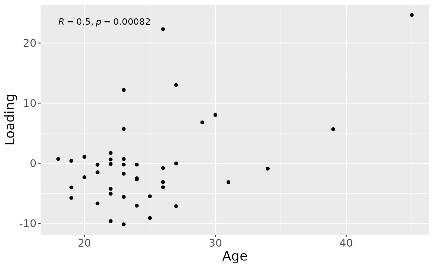
b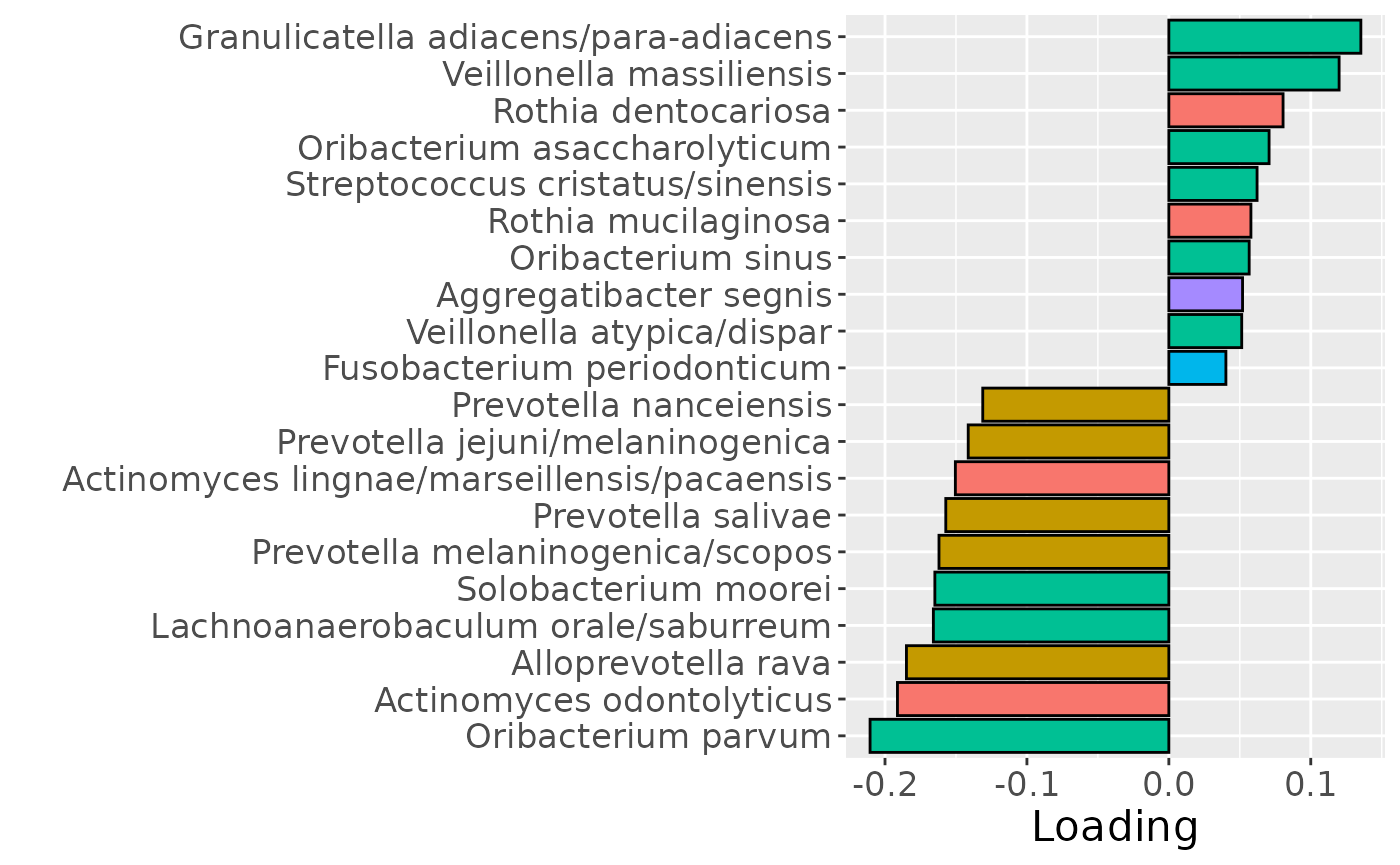
c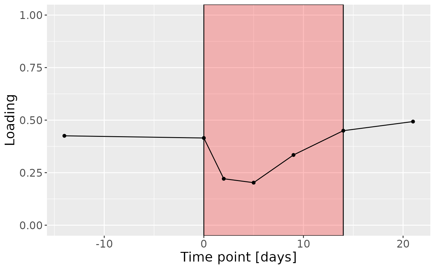
Positively loaded microbiota including Peptostreptococcus stomatis, Veillonella massiliensis, Porphyromonas pasteri, Lachnoanaerobaculum cf., Oribacterium parvum, Fusobacterium periodonticum, Aggregatibacter segnis, Granulicatella elegans, Capnocytophaga leadbetteri, and Veillonella parvula / rogosae / tobetsuensis were enriched in high responders and depleted in low responders. Conversely, negatively loaded microbiota including Prevotella jejuni / melaninogenica, Rothia dentocariosa, Streptococcus cristatus / sinensis, Veillonella atypica / dispar, Prevotella melaninogenica / scopos, Stomatobaculum longum, Rothia mucilaginosa, Actinomyces odontolyticus, Prevotella salivae, and Prevotella veroralis were enriched in low responders and depleted in high responders. The time mode loadings of the component indicated that inter-subject differences due to RF% were relatively constant, but transiently decreased during the intervention.
Lower jaw lingual microbiome
NPLS was subsequently applied to supervise the decomposition using the percentage of sites that were covered in red fluorescent plaque (RF%) as the dependent variable (y). The model selection procedure revealed that two components corresponded to the RMSECV minimum, explaining 13.2% of variation in X and 73.9% of variation in y, respectively. The commented code below performs the procedure, and is not rerun here due to computational limitations.
# CV_lowling = NPLStoolbox::ncrossreg(processedLowling$data, Ycnt, maxNumComponents = 10)
# a=CV_lowling$varExp %>% pivot_longer(-numComponents) %>% ggplot(aes(x=as.factor(numComponents),y=value,col=as.factor(name),group=as.factor(name))) + geom_line() + geom_point() + xlab("Number of components") + ylab("Variance explained (%)") + theme(legend.position="none")
# b=CV_lowling$RMSE %>% ggplot(aes(x=as.factor(numComponents),y=RMSE,group=1)) + geom_line() + geom_point() + xlab("Number of components") + ylab("RMSECV")
# ggarrange(a,b)
# npls_lowling = NPLStoolbox::triPLS1(processedLowling$data, Ycnt, 2)
npls_lowling = readRDS("./TIFN2/NPLS_lowling.RDS")

npls_lowling$varExpX
#> [1] 13.27838
npls_lowling$varExpY
#> [1] 73.93845
As expected, the first NPLS component captured variation exclusively associated with RF%, while the second component captured variation exclusively associated with subject gender.
testMetadata(npls_lowling, 1, processedLowling)
#>             Term  Estimate                                          CI
#> 1  plaquepercent  3.715363 -0.000645113811345087 – 0.00807583996130901
#> 2    bomppercent  2.342250 -0.000382021577102148 – 0.00506652135078373
#> 3 Area_delta_R30 13.104425    0.00761071083531463 – 0.0185981388922776
#> 4         gender 73.153268    -0.00420146304171221 – 0.150507999448965
#> 5            age  2.369166  -0.00452078411448064 – 0.00925911597240414
#>        P_value     P_adjust
#> 1 9.248392e-02 0.1156049046
#> 2 8.968515e-02 0.1156049046
#> 3 2.579248e-05 0.0001289624
#> 4 6.305775e-02 0.1156049046
#> 5 4.897460e-01 0.4897460333
testMetadata(npls_lowling, 2, processedLowling)
#>             Term    Estimate                                         CI
#> 1  plaquepercent   -4.114017  -0.0101326963347122 – 0.00190466133665912
#> 2    bomppercent   -2.165860 -0.00592611691772569 – 0.00159439766365394
#> 3 Area_delta_R30    1.603245 -0.00597961861614078 – 0.00918610807591475
#> 4         gender -108.454959  -0.215226144055683 – -0.00168377429959159
#> 5            age   -2.999926  -0.0125099860507945 – 0.00651013380601685
#>      P_value  P_adjust
#> 1 0.17401162 0.4169640
#> 2 0.25017839 0.4169640
#> 3 0.67038968 0.6703897
#> 4 0.04668113 0.2334057
#> 5 0.52608794 0.6576099
testFeatures(npls_lowling, processedLowling, 1, "Area_delta_R30") # flip
#> Joining with `by = join_by(subject, RFgroup)`
#> Joining with `by = join_by(subject, age, gender)`
#> [1] "Positive loadings:"
#>      Area_delta_R30
#> [1,]     -0.6772569
#> [1] "Negative loadings:"
#>      Area_delta_R30
#> [1,]      0.6772569

a = processedLowling$mode1 %>%
  mutate(Component_1 = npls_lowling$Fac[[1]][,1]) %>%
  left_join(rf_data %>% select(subject,day,Area_delta_R30,plaquepercent,bomppercent) %>% filter(day==14), by="subject") %>%
  ggplot(aes(x=Area_delta_R30,y=Component_1)) +
  geom_point() +
  xlab("RF%") +
  ylab("Loading") +
  stat_cor() +
  theme(text=element_text(size=16))

b = plotFeatures(processedLowling$mode2, npls_lowling, 1, flip=TRUE) + scale_fill_manual(values=phylum_colors[-7]) + theme(legend.position="none")

c = processedLowling$mode3 %>%
  mutate(Component_1 = -1*npls_lowling$Fac[[3]][,1], day=c(-14,0,2,5,9,14,21)) %>%
  ggplot(aes(x=day,y=Component_1)) +
  annotate(geom = "rect", xmin = 0, xmax = 14, ymin = -Inf, ymax = Inf, fill = "red", colour = "black", alpha=0.25) +
  geom_line() +
  geom_point() +
  xlab("Time point [days]") +
  ylab("Loading") +
  ylim(0,1) +
  theme(legend.position="none", text=element_text(size=16))

a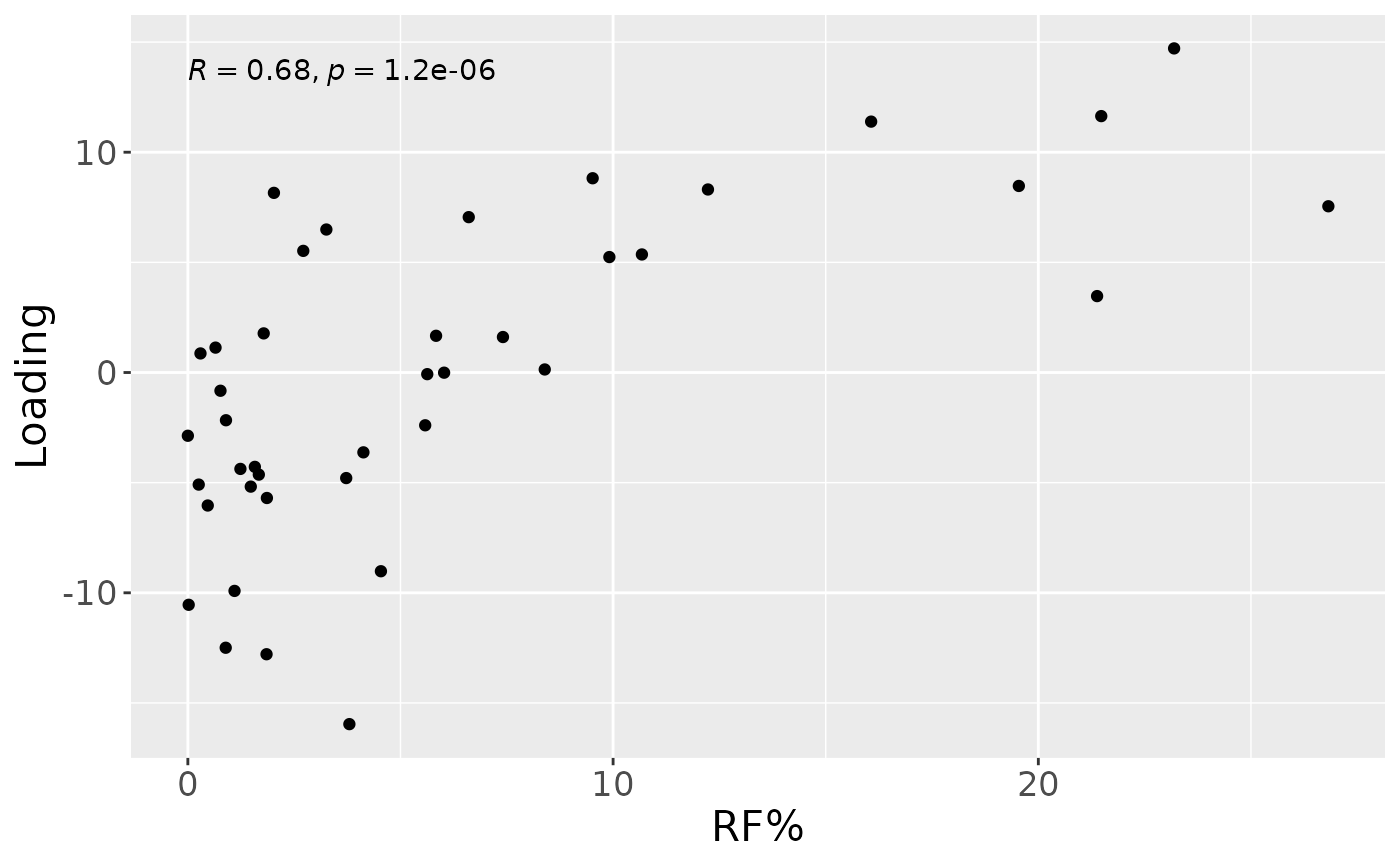
b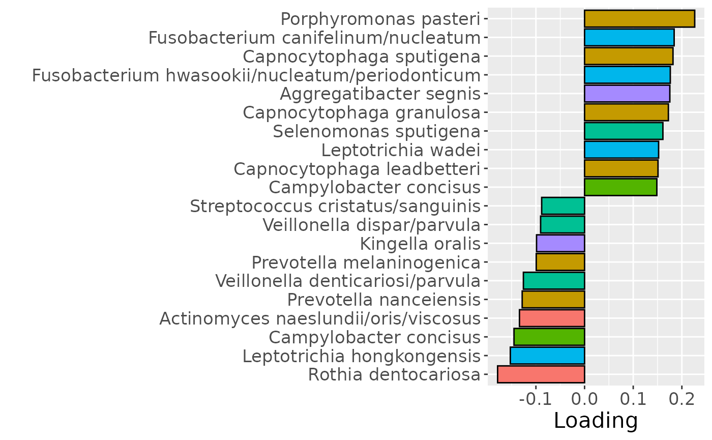
c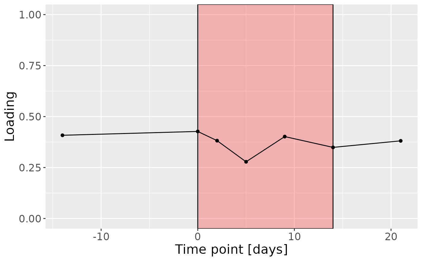
testFeatures(npls_lowling, processedLowling, 2, "gender") # no flip
#> Joining with `by = join_by(subject, RFgroup)`
#> Joining with `by = join_by(subject, age, gender)`
#> [1] "Positive loadings:"
#>         gender
#> [1,] 0.2793231
#> [1] "Negative loadings:"
#>          gender
#> [1,] -0.2793231

a = processedLowling$mode1 %>%
  mutate(Component_1 = npls_lowling$Fac[[1]][,2]) %>%
  left_join(rf_data %>% select(subject,day,Area_delta_R30,plaquepercent,bomppercent) %>% filter(day==14), by="subject") %>%
  ggplot(aes(x=as.factor(gender),y=Component_1)) +
  geom_boxplot() +
  xlab("Gender") +
  ylab("Loading") +
  scale_x_discrete(labels=c("Male","Female")) +
  theme(text=element_text(size=16))

b = plotFeatures(processedLowling$mode2, npls_lowling, 2, flip=FALSE) + scale_fill_manual(values=phylum_colors[-7]) + theme(legend.position="none")

c = processedLowling$mode3 %>%
  mutate(Component_1 = -1*npls_lowling$Fac[[3]][,2], day=c(-14,0,2,5,9,14,21)) %>%
  ggplot(aes(x=day,y=Component_1)) +
  annotate(geom = "rect", xmin = 0, xmax = 14, ymin = -Inf, ymax = Inf, fill = "red", colour = "black", alpha=0.25) +
  geom_line() +
  geom_point() +
  xlab("Time point [days]") +
  ylab("Loading") +
  ylim(0,1) +
  theme(legend.position="none", text=element_text(size=16))

a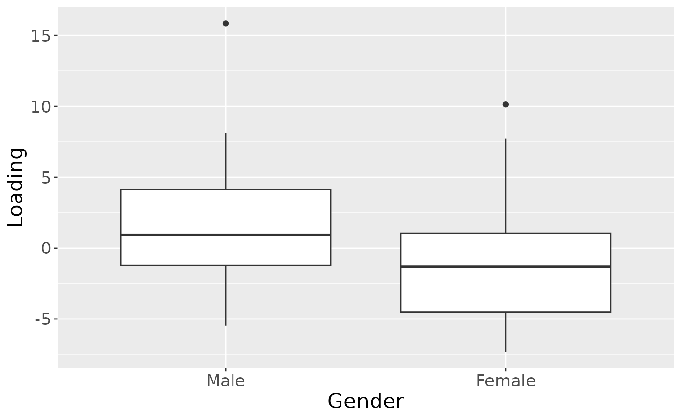
b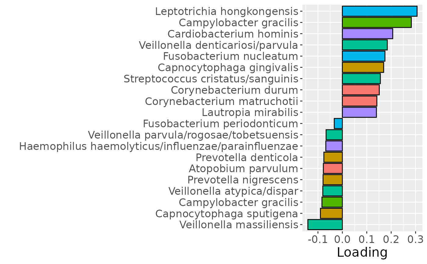
c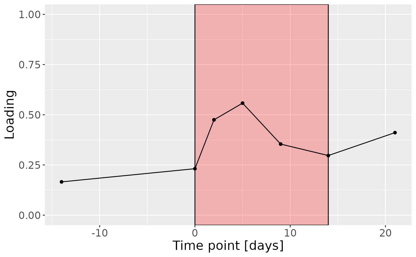
Lower jaw interproximal microbiome
NPLS was subsequently applied to supervise the decomposition using the percentage of sites that were covered in red fluorescent plaque (RF%) as dependent variable (y). The model selection procedure revealed that three components were appropriate due to a marked improvement in RMSECV, explaining 9.8% of variation in X and 94.0% of variation in y, respectively. The commented code below performs the procedure, and is not rerun here due to computational limitations.
# CV_lowinter = NPLStoolbox::ncrossreg(processedLowinter$data, Ycnt, maxNumComponents = 10)
# a=CV_lowinter$varExp %>% pivot_longer(-numComponents) %>% ggplot(aes(x=as.factor(numComponents),y=value,col=as.factor(name),group=as.factor(name))) + geom_line() + geom_point() + xlab("Number of components") + ylab("Variance explained (%)") + theme(legend.position="none")
# b=CV_lowinter$RMSE %>% ggplot(aes(x=as.factor(numComponents),y=RMSE,group=1)) + geom_line() + geom_point() + xlab("Number of components") + ylab("RMSECV")
# ggarrange(a,b)
# npls_lowinter = NPLStoolbox::triPLS1(processedLowinter$data, Ycnt, 3)
npls_lowinter = readRDS("./TIFN2/NPLS_lowinter.RDS")

npls_lowinter$varExpX
#> [1] 9.792967
npls_lowinter$varExpY
#> [1] 93.98916
As expected, the first NPLS component captured variation exclusively associated with RF%, while the second and third components were not interpretable.
testMetadata(npls_lowinter, 1, processedLowinter)
#>             Term   Estimate                                         CI
#> 1  plaquepercent  3.3096526 -0.00145265904366952 – 0.00807196416821377
#> 2    bomppercent -0.8384309 -0.00381375443174476 – 0.00213689268722177
#> 3 Area_delta_R30 15.2208403   0.00922085935199349 – 0.0212208211724995
#> 4         gender 69.1352412    -0.0153480260964937 – 0.153618508522373
#> 5            age  2.8573140  -0.00466757148278084 – 0.0103821994077065
#>        P_value     P_adjust
#> 1 1.671132e-01 2.785220e-01
#> 2 5.709283e-01 5.709283e-01
#> 3 1.019151e-05 5.095753e-05
#> 4 1.055865e-01 2.639664e-01
#> 5 4.459610e-01 5.574513e-01
testMetadata(npls_lowinter, 2, processedLowinter)
#>             Term    Estimate                                         CI
#> 1  plaquepercent  -4.0343329  -0.0103961845528384 – 0.00232751885082657
#> 2    bomppercent   1.5868511   -0.002387808391622 – 0.00556151068560298
#> 3 Area_delta_R30  -0.7891306 -0.00880435348664343 – 0.00722609219743649
#> 4         gender -79.4547914    -0.192313852803302 – 0.0334042699832537
#> 5            age  -5.6192399  -0.0156715441175292 – 0.00443306441593625
#>     P_value  P_adjust
#> 1 0.2064097 0.4402644
#> 2 0.4231274 0.5289092
#> 3 0.8427373 0.8427373
#> 4 0.1618029 0.4402644
#> 5 0.2641586 0.4402644
testMetadata(npls_lowinter, 3, processedLowinter)
#>             Term    Estimate                                         CI
#> 1  plaquepercent   1.9616635 -0.00441084473003135 – 0.00833417182067836
#> 2    bomppercent  -2.5562100 -0.00653752736785625 – 0.00142510740850312
#> 3 Area_delta_R30  -0.7397026 -0.00876835152455174 – 0.00728894634518655
#> 4         gender -38.8830025     -0.15193111123446 – 0.0741651061515203
#> 5            age   5.9104434   -0.0041586991794963 – 0.0159795860646214
#>     P_value  P_adjust
#> 1 0.5360685 0.6700857
#> 2 0.2009361 0.6035466
#> 3 0.8527095 0.8527095
#> 4 0.4896298 0.6700857
#> 5 0.2414186 0.6035466
testFeatures(npls_lowinter, processedLowinter, 1, "Area_delta_R30") # NO flip
#> Joining with `by = join_by(subject, RFgroup)`
#> Joining with `by = join_by(subject, age, gender)`
#> [1] "Positive loadings:"
#>      Area_delta_R30
#> [1,]      0.7072254
#> [1] "Negative loadings:"
#>      Area_delta_R30
#> [1,]     -0.7072254

a = processedLowinter$mode1 %>%
  mutate(Component_1 = npls_lowinter$Fac[[1]][,1]) %>%
  left_join(rf_data %>% select(subject,day,Area_delta_R30,plaquepercent,bomppercent) %>% filter(day==14), by="subject") %>%
  ggplot(aes(x=Area_delta_R30,y=Component_1)) +
  geom_point() +
  xlab("RF%") +
  ylab("Loading") +
  stat_cor() +
  theme(text=element_text(size=16))

b = plotFeatures(processedLowinter$mode2, npls_lowinter, 1, flip=FALSE) + scale_fill_manual(values=phylum_colors[-7]) + theme(legend.position="none")

c = processedLowinter$mode3 %>%
  mutate(Component_1 = npls_lowinter$Fac[[3]][,1], day=c(-14,0,2,5,9,14,21)) %>%
  ggplot(aes(x=day,y=Component_1)) +
  annotate(geom = "rect", xmin = 0, xmax = 14, ymin = -Inf, ymax = Inf, fill = "red", colour = "black", alpha=0.25) +
  geom_line() +
  geom_point() +
  xlab("Time point [days]") +
  ylab("Loading") +
  ylim(0,1) +
  theme(legend.position="none", text=element_text(size=16))

a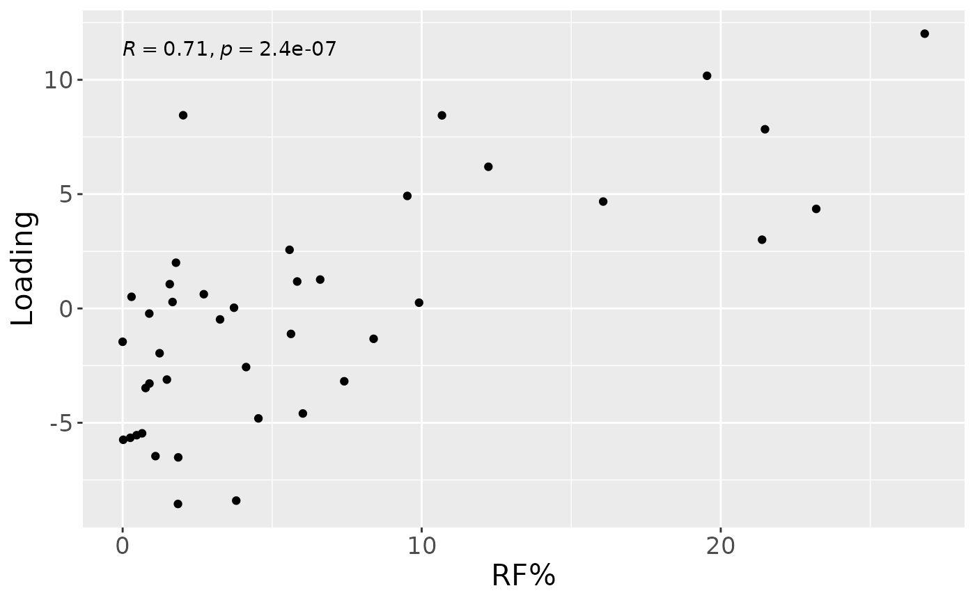
b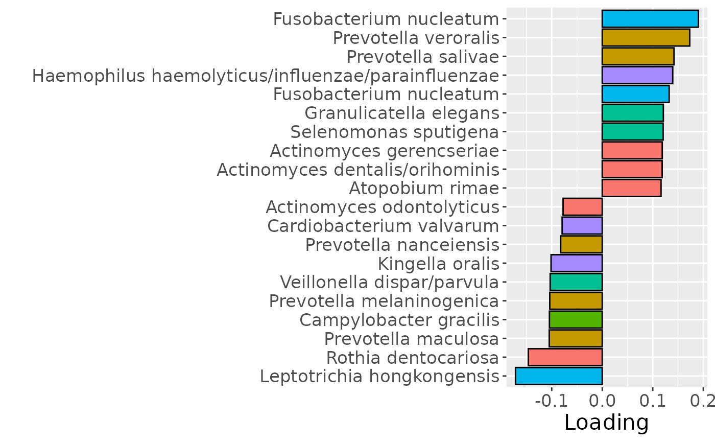
c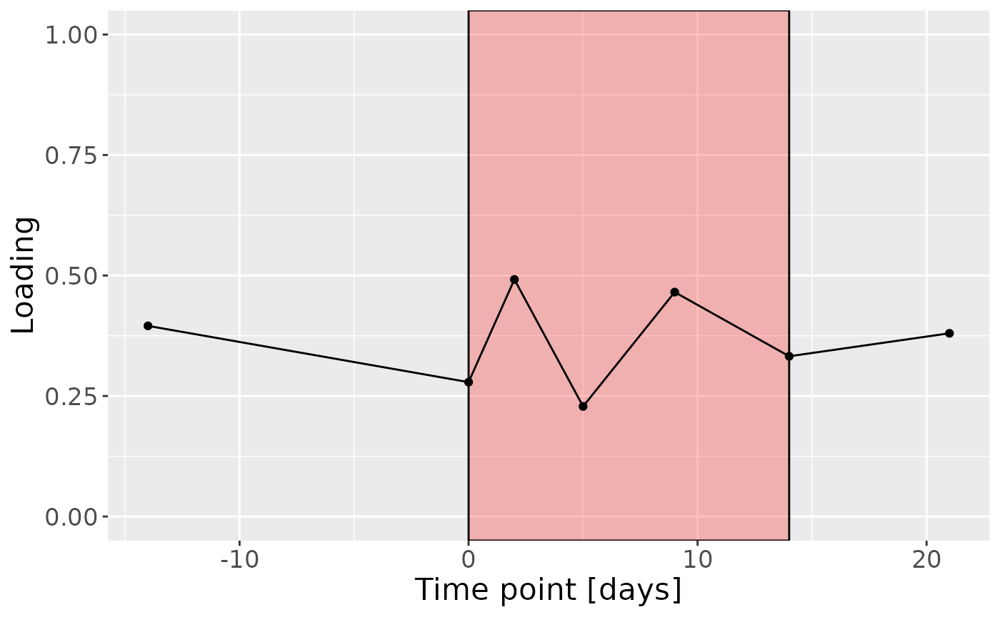
Positively loaded microbiota including Fusobacterium nucleatum, Prevotella veroralis, Prevotella salivae, Haemophilus haemolyticus / influenzae / parainfluenzae, Granulicatella elegans, Selenomonas sputigena, Actinomyces gerencseriae, Actinomyces dentalis / orihominis, and Atopobium rimae were enriched in high responders and depleted in low responders. Conversely, negatively loaded microbiota including Leptotrichia hongkongensis, Rothia dentocariosa, Prevotella maculosa, Campylobacter gracilis, Prevotella melaninogenica, Veillonella dispar / parvula, Kingella oralis, Prevotella nanceiensis, Cardiobacterium valvarum, and Actinomyces odontolyticus were enriched in low responders and depleted in high responders. The time mode loadings did not reveal any clear temporal pattern.
Upper jaw lingual microbiome
NPLS was subsequently applied to supervise the decomposition using the percentage of sites that were covered in red fluorescent plaque (RF%) as dependent variable (y). The model selection procedure revealed that one component corresponded to the RMSECV minimum, explaining 7.1% of variation in X and 37.3% of variation in y. The commented code below performs the procedure, and is not rerun here due to computational limitations.
# CV_upling = NPLStoolbox::ncrossreg(processedUpling$data, Ycnt, maxNumComponents = 10)
# a=CV_upling$varExp %>% pivot_longer(-numComponents) %>% ggplot(aes(x=as.factor(numComponents),y=value,col=as.factor(name),group=as.factor(name))) + geom_line() + geom_point() + xlab("Number of components") + ylab("Variance explained (%)") + theme(legend.position="none")
# b=CV_upling$RMSE %>% ggplot(aes(x=as.factor(numComponents),y=RMSE,group=1)) + geom_line() + geom_point() + xlab("Number of components") + ylab("RMSECV")
# ggarrange(a,b)
# npls_upling = NPLStoolbox::triPLS1(processedUpling$data, Ycnt, 1)
npls_upling = readRDS("./TIFN2/NPLS_upling.RDS")

npls_upling$varExpX
#> [1] 7.050193
npls_upling$varExpY
#> [1] 37.33265
As expected, MLR analysis revealed that the NPLS component captured variation exclusively associated with RF%.
testMetadata(npls_upling, 1, processedUpling)
#>             Term   Estimate                                          CI
#> 1  plaquepercent  4.0478033 -0.000770578431992336 – 0.00886618505872002
#> 2    bomppercent  1.2401645  -0.00177018966493134 – 0.00425051872704196
#> 3 Area_delta_R30 13.2165671    0.00714594404762599 – 0.0192871900989676
#> 4         gender 74.4980064     -0.0109799434918638 – 0.159975956363131
#> 5            age -0.7702828  -0.00838376420630882 – 0.00684319852331261
#>        P_value     P_adjust
#> 1 9.697323e-02 0.1616220476
#> 2 4.086397e-01 0.5107996315
#> 3 9.122167e-05 0.0004561084
#> 4 8.555172e-02 0.1616220476
#> 5 8.384549e-01 0.8384548793
model = npls_upling
df = processedUpling

testFeatures(model, df, 1, "Area_delta_R30") # NO flip
#> Joining with `by = join_by(subject, RFgroup)`
#> Joining with `by = join_by(subject, age, gender)`
#> [1] "Positive loadings:"
#>      Area_delta_R30
#> [1,]      0.6110045
#> [1] "Negative loadings:"
#>      Area_delta_R30
#> [1,]     -0.6110045

a = df$mode1 %>%
  mutate(Component_1 = model$Fac[[1]][,1]) %>%
  left_join(rf_data %>% select(subject,day,Area_delta_R30,plaquepercent,bomppercent) %>% filter(day==14), by="subject") %>%
  ggplot(aes(x=Area_delta_R30,y=Component_1)) +
  geom_point() +
  xlab("RF%") +
  ylab("Loading") +
  stat_cor() +
  theme(text=element_text(size=16))

b = plotFeatures(df$mode2, model, 1, flip=FALSE) + scale_fill_manual(values=phylum_colors[-c(3,7)]) + theme(legend.position="none")

c = df$mode3 %>%
  mutate(Component_1 = model$Fac[[3]][,1], day=c(-14,0,2,5,9,14,21)) %>%
  ggplot(aes(x=day,y=Component_1)) +
  annotate(geom = "rect", xmin = 0, xmax = 14, ymin = -Inf, ymax = Inf, fill = "red", colour = "black", alpha=0.25) +
  geom_line() +
  geom_point() +
  xlab("Time point [days]") +
  ylab("Loading") +
  ylim(0,1) +
  theme(legend.position="none", text=element_text(size=16))

a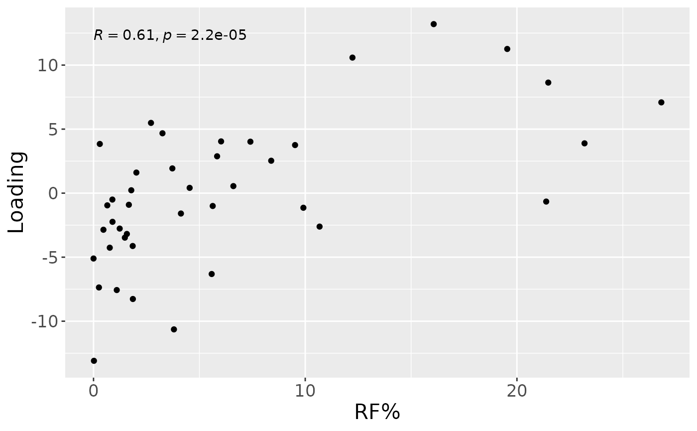
b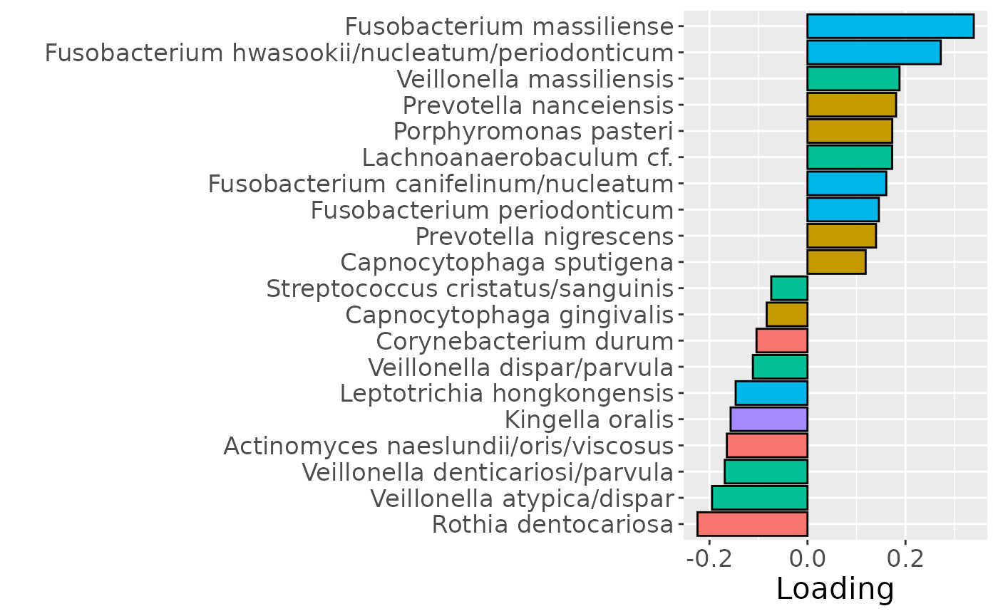
c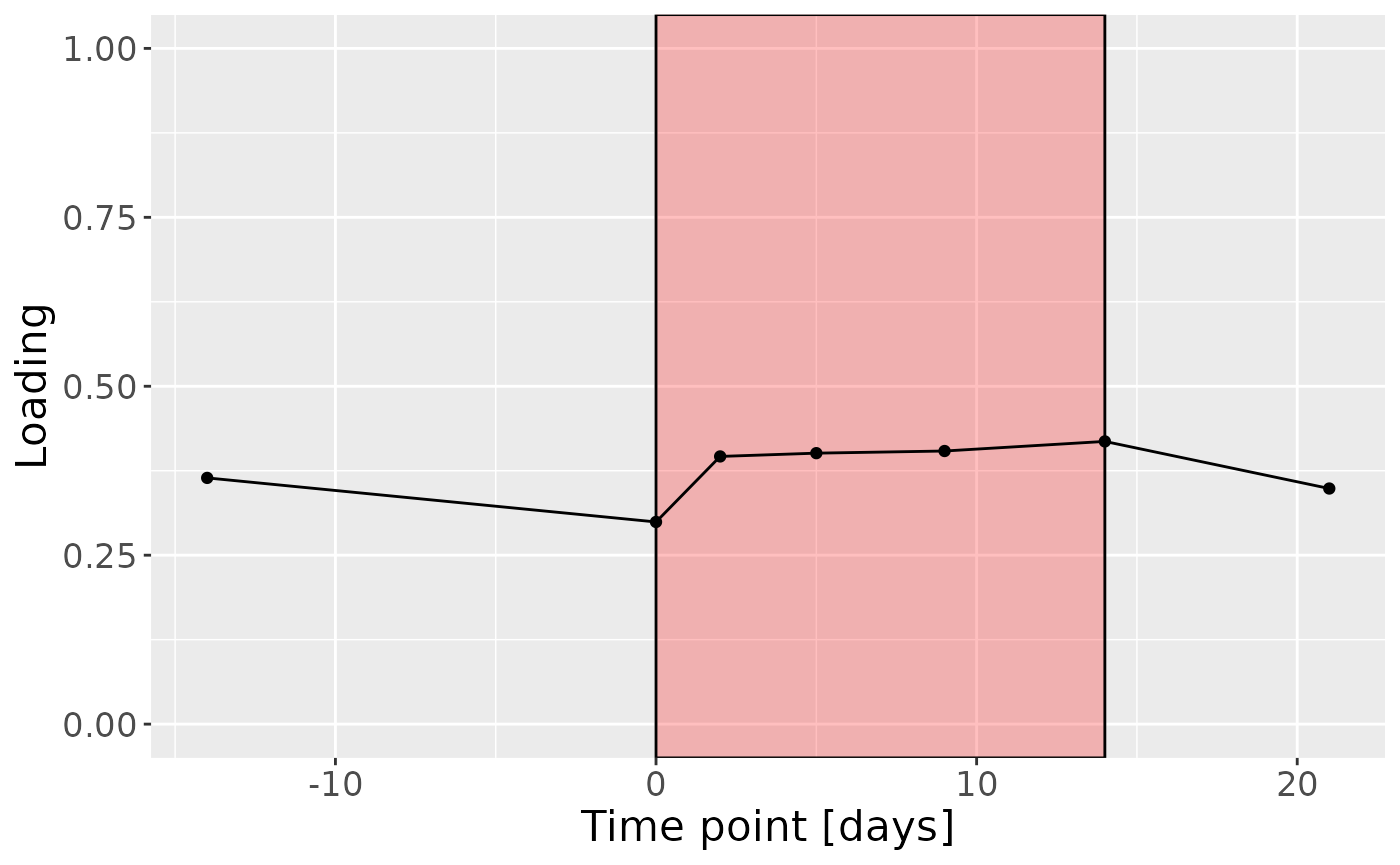
Positively loaded microbiota including Fusobacterium massiliense, Fusobacterium hwasookii / nucleatum / periodonticum, Veillonella massiliensis, Prevotella nanceiensis, Porphyromonas pasteri, Lachnoanaerobaculum cf., Fusobacterium canifelinum / nucleatum, Fusobacterium periodonticum, Prevotella nigrescens, and Capnocytophaga sputigena were enriched in high responders and depleted in low responders. Conversely, negatively loaded microbiota including Rothia dentocariosa, Veillonella atypica / dispar, Veillonella denticariosi / parvula, Actinomyces naeslundii / oris / viscosus, Kingella oris, Leptotrichia hongkongensis, Veillonella dispar / parvula, Corynebacterium durum, Capnocytophaga gingivalis, and Streptococcus cristatus / sanguinis were enriched in low responders and depleted in high responders. The time mode loadings showed a transient increase in inter-subject differences during the intervention period.
Upper jaw interproximal microbiome
NPLS was subsequently applied to supervise the decomposition using the percentage of sites that were covered in red fluorescent plaque (RF%) as dependent variable (y). The model selection procedure revealed that one component corresponded to an RMSECV minimum, explaining 6.4% of variation in X and 34.3% of variation in y. The commented code below performs the procedure, and is not rerun here due to computational limitations.
# CV_upinter = NPLStoolbox::ncrossreg(processedUpinter$data, Ycnt, maxNumComponents = 10)
# a=CV_upinter$varExp %>% pivot_longer(-numComponents) %>% ggplot(aes(x=as.factor(numComponents),y=value,col=as.factor(name),group=as.factor(name))) + geom_line() + geom_point() + xlab("Number of components") + ylab("Variance explained (%)") + theme(legend.position="none")
# b=CV_upinter$RMSE %>% ggplot(aes(x=as.factor(numComponents),y=RMSE,group=1)) + geom_line() + geom_point() + xlab("Number of components") + ylab("RMSECV")
# ggarrange(a,b)
# npls_upinter = NPLStoolbox::triPLS1(processedUpinter$data, Ycnt, 1)
npls_upinter = readRDS("./TIFN2/NPLS_upinter.RDS")

npls_upinter$varExpX
#> [1] 6.360512
npls_upinter$varExpY
#> [1] 34.30872
As expected, MLR analysis revealed that the NPLS component captured variation exclusively associated with RF%.
testMetadata(npls_upinter, 1, processedUpinter)
#>             Term  Estimate                                          CI
#> 1  plaquepercent  3.339033  -0.00145139242610112 – 0.00812945878601939
#> 2    bomppercent  2.408691 -0.000584197467843378 – 0.00540157891347544
#> 3 Area_delta_R30 11.841794    0.00580639255553114 – 0.0178771953784663
#> 4         gender 81.810902     -0.00317110717769579 – 0.16679291050557
#> 5            age  1.978115  -0.00559119347772117 – 0.00954742276678969
#>        P_value    P_adjust
#> 1 0.1658958036 0.207369755
#> 2 0.1112570321 0.185428387
#> 3 0.0003277558 0.001638779
#> 4 0.0586855593 0.146713898
#> 5 0.5990911027 0.599091103
model = npls_upinter
df = processedUpinter

testFeatures(model, df, 1, "Area_delta_R30") # NO flip
#> Joining with `by = join_by(subject, RFgroup)`
#> Joining with `by = join_by(subject, age, gender)`
#> [1] "Positive loadings:"
#>      Area_delta_R30
#> [1,]      0.5857467
#> [1] "Negative loadings:"
#>      Area_delta_R30
#> [1,]     -0.5857467

a = df$mode1 %>%
  mutate(Component_1 = model$Fac[[1]][,1]) %>%
  left_join(rf_data %>% select(subject,day,Area_delta_R30,plaquepercent,bomppercent) %>% filter(day==14), by="subject") %>%
  ggplot(aes(x=Area_delta_R30,y=Component_1)) +
  geom_point() +
  xlab("RF%") +
  ylab("Loading") +
  stat_cor() +
  theme(text=element_text(size=16))

b = plotFeatures(df$mode2, model, 1, flip=FALSE) + scale_fill_manual(values=phylum_colors[-c(3,7)]) + theme(legend.position="none")

c = df$mode3 %>%
  mutate(Component_1 = model$Fac[[3]][,1], day=c(-14,0,2,5,9,14,21)) %>%
  ggplot(aes(x=day,y=Component_1)) +
  annotate(geom = "rect", xmin = 0, xmax = 14, ymin = -Inf, ymax = Inf, fill = "red", colour = "black", alpha=0.25) +
  geom_line() +
  geom_point() +
  xlab("Time point [days]") +
  ylab("Loading") +
  ylim(0,1) +
  theme(legend.position="none", text=element_text(size=16))

a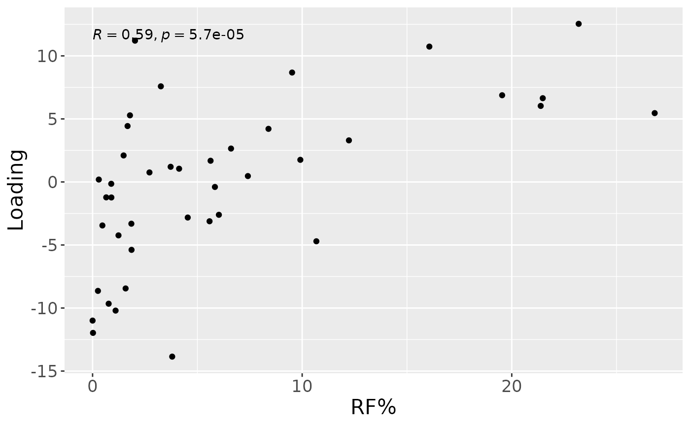
b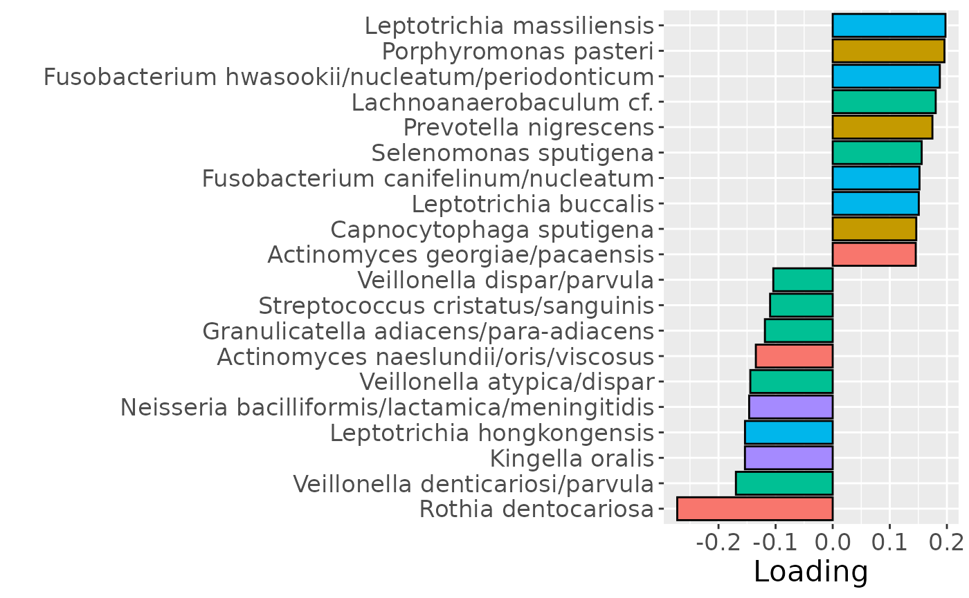
c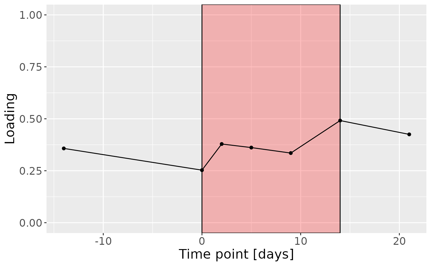
Positively loaded microbiota including Leptotrichia massiliensis, Porphyromonas pasteri, Fusobacterium hwasookii / nucleatum / periodonticum, Lachnoanaerobaculum cf., Prevotella nigrescens, Selenomonas sputigena, Fusobacterium canifelinum / nucleatum, Leptotrichia buccalis, Capnocytophaga sputigena, and Actinomyces georgiae / pacaensis were enriched in high responders and depleted in low responders. Conversely, negatively loaded microbiota including Rothia dentocariosa, Veillonella denticariosi / parvula, Kingella oralis, Leptotrichia hongkongensis, Neisseria bacilliformis / lactamica / meningitidis, Veillonella atypica / dispar, Actinomyces naeslundii / oris / viscosus, Granulicatella adiacens / para-adiacens, Streptococcus cristatus / sanguinis, and Veillonella dispar / parvula were enriched in low responders and depleted in high responders. The time mode loadings indicated that inter-subject differences increased over time, reaching a maximum at day 14.
Salivary microbiome
NPLS was subsequently applied to supervise the decomposition using the percentage of sites that were covered in red fluorescent plaque (RF%) as dependent variable (y). The model selection procedure revealed that one component corresponded to the RMSECV minimum, explaining 5.2% of variation in X and 33.2% of variation in y, respectively. The commented code below performs the procedure, and is not rerun here due to computational limitations.
# CV_saliva = NPLStoolbox::ncrossreg(processedSaliva$data, Ycnt, maxNumComponents = 10)
# a=CV_saliva$varExp %>% pivot_longer(-numComponents) %>% ggplot(aes(x=as.factor(numComponents),y=value,col=as.factor(name),group=as.factor(name))) + geom_line() + geom_point() + xlab("Number of components") + ylab("Variance explained (%)") + theme(legend.position="none")
# b=CV_saliva$RMSE %>% ggplot(aes(x=as.factor(numComponents),y=RMSE,group=1)) + geom_line() + geom_point() + xlab("Number of components") + ylab("RMSECV")
# ggarrange(a,b)
# npls_saliva = NPLStoolbox::triPLS1(processedSaliva$data, Ycnt, 1)
npls_saliva = readRDS("./TIFN2/NPLS_saliva.RDS")

npls_saliva$varExpX
#> [1] 5.179739
npls_saliva$varExpY
#> [1] 33.22421
As expected, MLR analysis revealed that the NPLS component captured variation exclusively associated with RF%.
testMetadata(npls_saliva, 1, processedSaliva)
#>             Term  Estimate                                          CI
#> 1  plaquepercent  0.517096  -0.00463103466799416 – 0.00566522660467623
#> 2    bomppercent  2.351534 -0.000864835629191632 – 0.00556790361049825
#> 3 Area_delta_R30 12.091719    0.00560564942822247 – 0.0185777890517456
#> 4         gender 66.576150     -0.0247515353456588 – 0.157903835693377
#> 5            age  2.281081   -0.00585343328619292 – 0.0104155959168686
#>        P_value    P_adjust
#> 1 0.8396040573 0.839604057
#> 2 0.1466959221 0.246404995
#> 3 0.0005792527 0.002896263
#> 4 0.1478429972 0.246404995
#> 5 0.5727997357 0.715999670
model = npls_saliva
df = processedSaliva

testFeatures(model, df, 1, "Area_delta_R30") # NO flip
#> Joining with `by = join_by(subject, RFgroup)`
#> Joining with `by = join_by(subject, age, gender)`
#> [1] "Positive loadings:"
#>      Area_delta_R30
#> [1,]      0.5764045
#> [1] "Negative loadings:"
#>      Area_delta_R30
#> [1,]     -0.5764045

a = df$mode1 %>%
  mutate(Component_1 = model$Fac[[1]][,1]) %>%
  left_join(rf_data %>% select(subject,day,Area_delta_R30,plaquepercent,bomppercent) %>% filter(day==14), by="subject") %>%
  ggplot(aes(x=Area_delta_R30,y=Component_1)) +
  geom_point() +
  xlab("RF%") +
  ylab("Loading") +
  stat_cor() +
  theme(text=element_text(size=16))

b = plotFeatures(df$mode2, model, 1, flip=FALSE) + scale_fill_manual(values=phylum_colors[-c(3,7)]) + theme(legend.position="none")

c = df$mode3 %>%
  mutate(Component_1 = model$Fac[[3]][,1], day=c(-14,0,2,5,9,14,21)) %>%
  ggplot(aes(x=day,y=Component_1)) +
  annotate(geom = "rect", xmin = 0, xmax = 14, ymin = -Inf, ymax = Inf, fill = "red", colour = "black", alpha=0.25) +
  geom_line() +
  geom_point() +
  xlab("Time point [days]") +
  ylab("Loading") +
  ylim(0,1) +
  theme(legend.position="none", text=element_text(size=16))

a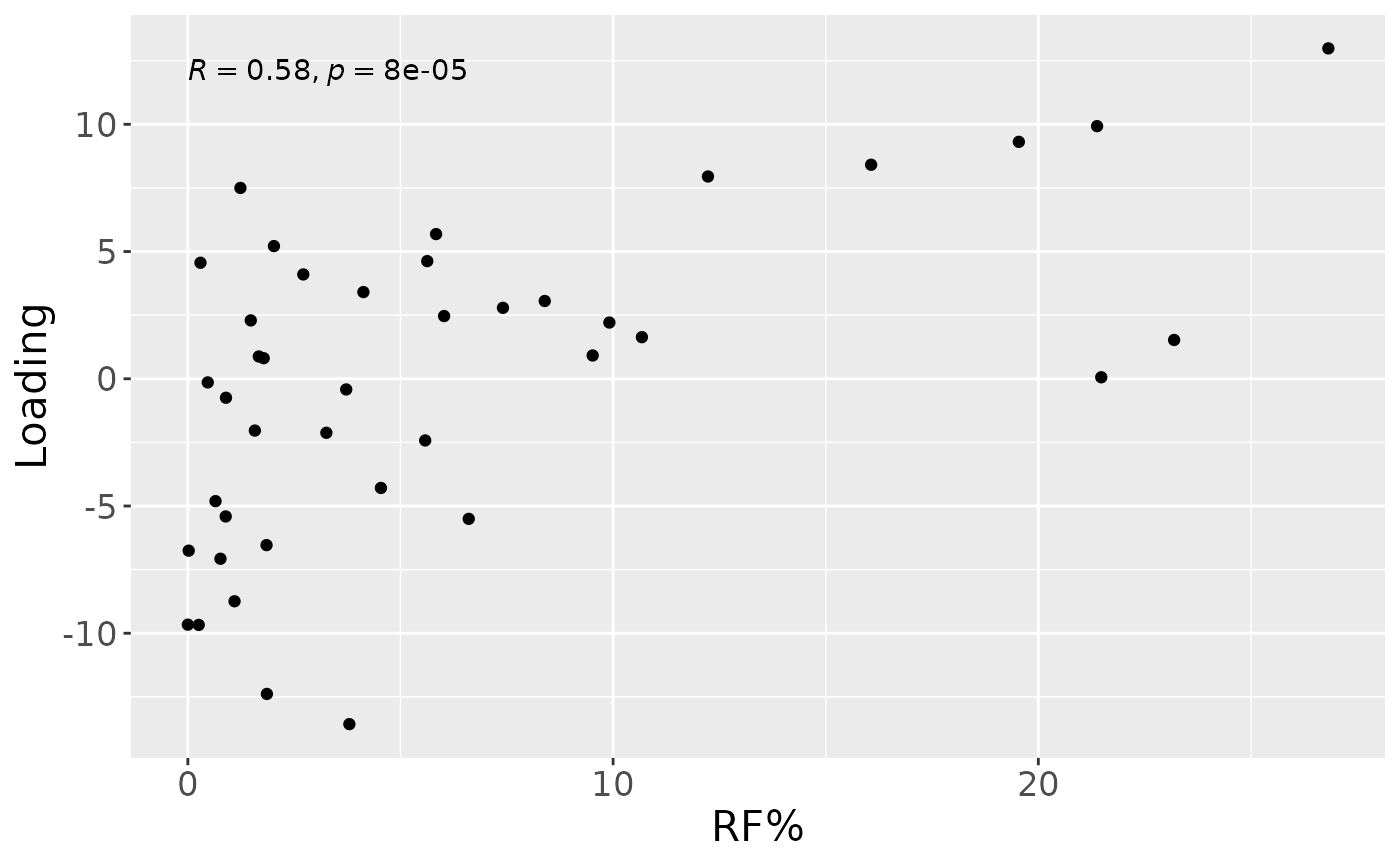
b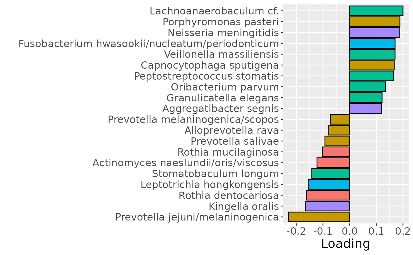
c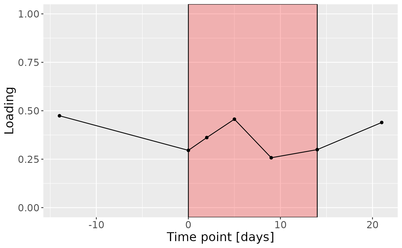
Positively loaded microbiota including Lachnoanaerobaculum cf., Porphyromonas pasteri, Neisseria meningitidis, Fusobacterium hwasookii / nucleatum / periodonticum, Veillonella massiliensis, Capnocytophaga sputigena, Peptostreptococcus stomatis, Oribacterium parvum, Granulicatella elegans, and Aggregatibacter segnis were enriched in high responders and depleted in low responders. Conversely, negatively loaded microbiota including Prevotella jejuni / melaninogenica, Kingella oralis, Rothia dentocariosa, Leptotrichia hongkongensis, Stomatobaculum longum, Actinomyces naeslundii / oris / viscosus, Rothia mucilaginosa, Prevotella salivae, Alloprevotella rava, and Prevotella melaninogenica / scopos were enriched in low responders and depleted in high responders. The time mode loadings showed a brief increase in inter-subject differences peaking around day 5, followed by a decline.
Salivary metabolomics
NPLS was subsequently applied to supervise the decomposition using the percentage of sites that were covered in red fluorescent plaque (RF%) as dependent variable (y). The model selection procedure revealed that one component corresponded to the RMSECV minimum, explaining 8.7% of variation in X and 25.7% of variation in y. The commented code below performs the procedure, and is not rerun here due to computational limitations.
# CV_metab = NPLStoolbox::ncrossreg(processedMetabolomics$data, Ymetab_cnt, maxNumComponents = 10)
# a=CV_metab$varExp %>% pivot_longer(-numComponents) %>% ggplot(aes(x=as.factor(numComponents),y=value,col=as.factor(name),group=as.factor(name))) + geom_line() + geom_point() + xlab("Number of components") + ylab("Variance explained (%)") + theme(legend.position="none")
# b=CV_metab$RMSE %>% ggplot(aes(x=as.factor(numComponents),y=RMSE,group=1)) + geom_line() + geom_point() + xlab("Number of components") + ylab("RMSECV")
# ggarrange(a,b)
# npls_metab = NPLStoolbox::triPLS1(processedMetabolomics$data, Ymetab_cnt, 1)
npls_metab = readRDS("./TIFN2/NPLS_metab.RDS")

npls_metab$varExpX
#> [1] 8.655991
npls_metab$varExpY
#> [1] 25.66813
As expected, MLR analysis revealed that the NPLS component captured variation exclusively associated with RF%.
testMetadata(npls_metab, 1, processedMetabolomics)
#>             Term   Estimate                                         CI
#> 1  plaquepercent   4.293501 -0.00105841095712955 – 0.00964541325008825
#> 2    bomppercent   2.176664 -0.00109724071284544 – 0.00545056969051656
#> 3 Area_delta_R30   9.022539   0.00241777824108076 – 0.0156272996462027
#> 4         gender -28.216210    -0.121348837973755 – 0.0649164180705563
#> 5            age  -5.708618  -0.0139889510436936 – 0.00257171604047823
#>       P_value   P_adjust
#> 1 0.112260095 0.23196582
#> 2 0.185572658 0.23196582
#> 3 0.008879154 0.04439577
#> 4 0.542189172 0.54218917
#> 5 0.170255737 0.23196582
model = npls_metab
df = processedMetabolomics

testFeatures(model, df, 1, "Area_delta_R30") # NO flip
#> Joining with `by = join_by(subject, RFgroup)`
#> Joining with `by = join_by(subject, age, gender)`
#> [1] "Positive loadings:"
#>      Area_delta_R30
#> [1,]      0.5066373
#> [1] "Negative loadings:"
#>      Area_delta_R30
#> [1,]     -0.5066373

a = df$mode1 %>%
  mutate(Component_1 = model$Fac[[1]][,1]) %>%
  left_join(rf_data %>% select(subject,day,Area_delta_R30,plaquepercent,bomppercent) %>% filter(day==14), by="subject") %>%
  ggplot(aes(x=Area_delta_R30,y=Component_1)) +
  geom_point() +
  xlab("RF%") +
  ylab("Loading") +
  stat_cor() +
  theme(text=element_text(size=16))

temp = processedMetabolomics$mode2 %>% mutate(Component_1 = npls_metab$Fac[[2]][,1]) %>% arrange(Component_1) %>% mutate(index=1:nrow(.))
temp = rbind(temp %>% head(n=10), temp %>% tail(n=10))

b = temp %>%
  ggplot(aes(x = Component_1, y = as.factor(index),
             fill = as.factor(Type),
             pattern = as.factor(Type))) +
  geom_bar_pattern(stat = "identity",
                   colour = "black",
                   pattern = "stripe",
                   pattern_fill = "black",
                   pattern_density = 0.2,
                   pattern_spacing = 0.05,
                   pattern_angle = 45,
                   pattern_size = 0.2) +
  scale_y_discrete(labels = temp$Name) +
  xlab("Loading") +
  ylab("") +
  guides(fill = guide_legend(title = "Class"),
         pattern = "none") +
  theme(text = element_text(size = 16),
        legend.position = "none")

c = df$mode3 %>%
  mutate(Component_1 = model$Fac[[3]][,1], day=c(0,2,5,9,14)) %>%
  ggplot(aes(x=day,y=Component_1)) +
  annotate(geom = "rect", xmin = 0, xmax = 14, ymin = -Inf, ymax = Inf, fill = "red", colour = "black", alpha=0.25) +
  geom_line() +
  geom_point() +
  xlab("Time point [days]") +
  ylab("Loading") +
  ylim(0,1) +
  theme(legend.position="none", text=element_text(size=16))

a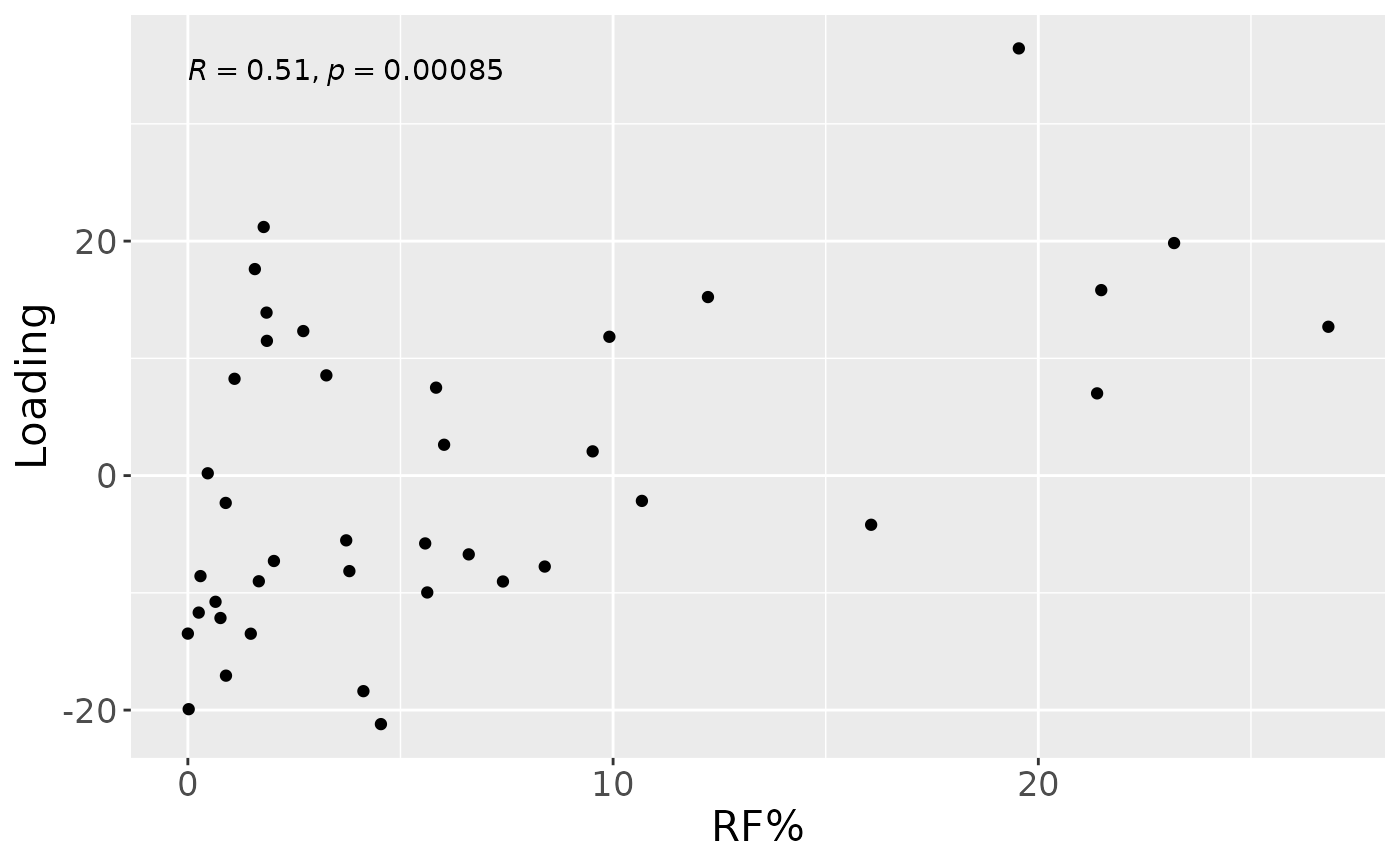
b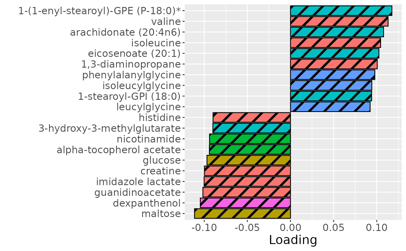
c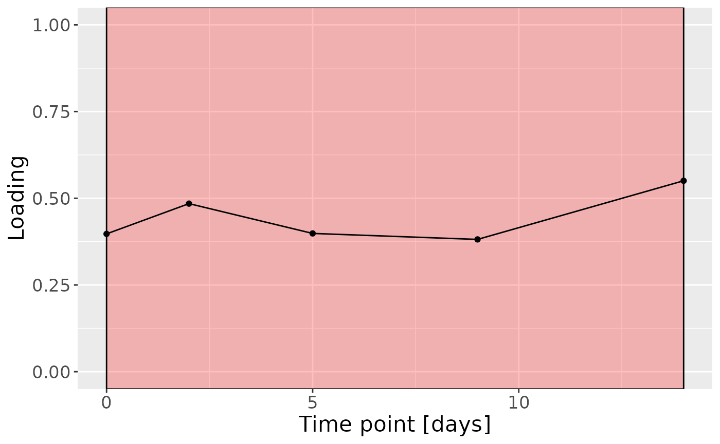
Higher RF% was associated with elevated levels of amino acids and dipeptides, including valine, isoleucine, and leucylglycine. In addition, increased concentrations of arachidonate, and polyamines including 1,3-diaminopropane, were observed in this group. Conversely, individuals with lower RF% exhibited higher levels of carbohydrates (e.g., maltose, glucose), energy-related compounds (e.g., creatine, guanidinoacetate), and vitamin-related metabolites such as nicotinamide, dexpanthenol, and alpha-tocopherol acetate. The time mode loadings indicated that inter-subject differences were maximal at day 14.