MAINHEALTH: intergenerational obesity transmission
2025-08-31
Source:vignettes/articles/MAINHEALTH.Rmd
MAINHEALTH.RmdIntroduction
This article presents the NPLS results of the MAINHEALTH dataset discussed in Chapter 5 of my dissertation.
Preamble
testMetadata = function(model, comp, metadata){
  transformedSubjectLoadings = model$Fac[[1]][,comp]
  transformedSubjectLoadings = transformedSubjectLoadings / norm(transformedSubjectLoadings, "2")

  result = lm(transformedSubjectLoadings ~ BMI + C.section + Secretor + Lewis + whz.6m, data=metadata$mode1)

  # Extract coefficients and confidence intervals
  coef_estimates <- summary(result)$coefficients
  conf_intervals <- confint(result)

  # Remove intercept
  coef_estimates <- coef_estimates[rownames(coef_estimates) != "(Intercept)", ]
  conf_intervals <- conf_intervals[rownames(conf_intervals) != "(Intercept)", ]

  # Combine into a clean data frame
  summary_table <- data.frame(
    Term     = rownames(coef_estimates),
    Estimate = coef_estimates[, "Estimate"] * 1e3,
    CI       = paste0(
                 conf_intervals[, 1], " – ",
                 conf_intervals[, 2]
               ),
    P_value  = coef_estimates[, "Pr(>|t|)"],
    P_adjust = p.adjust(coef_estimates[, "Pr(>|t|)"], "BH"),
    row.names = NULL
  )

  return(summary_table)
}
colours = RColorBrewer:: brewer.pal(8, "Dark2")
BMI_cols = c("darkgreen","darkgoldenrod","darkred") #colours[1:3]
WHZ_cols = c("darkgreen", "darkgoldenrod", "dodgerblue4")
phylum_cols = colours
Maternal pre-pregnancy BMI
Processing
# Faeces
newFaeces = NPLStoolbox::Jakobsen2025$faeces

mask = newFaeces$mode1$subject %in% (NPLStoolbox::Jakobsen2025$faeces$mode1 %>% filter(!is.na(BMI)) %>% select(subject) %>% pull())
newFaeces$data = newFaeces$data[mask,,]
newFaeces$mode1 = newFaeces$mode1[mask,]
processedFaeces = parafac4microbiome::processDataCube(newFaeces, sparsityThreshold = 0.75, centerMode=1, scaleMode=2)

# Milk
newMilk = NPLStoolbox::Jakobsen2025$milkMicrobiome

mask = newMilk$mode1$subject %in% (NPLStoolbox::Jakobsen2025$milkMicrobiome$mode1 %>% filter(!is.na(BMI)) %>% select(subject) %>% pull())
newMilk$data = newMilk$data[mask,,]
newMilk$mode1 = newMilk$mode1[mask,]
processedMilk = parafac4microbiome::processDataCube(newMilk, sparsityThreshold=0.85, centerMode=1, scaleMode=2)

# Milk metab
newMilkMetab = NPLStoolbox::Jakobsen2025$milkMetabolomics

mask = newMilkMetab$mode1$subject %in% (NPLStoolbox::Jakobsen2025$milkMetabolomics$mode1 %>% filter(!is.na(BMI)) %>% select(subject) %>% pull())
newMilkMetab$data = newMilkMetab$data[mask,,]
newMilkMetab$mode1 = newMilkMetab$mode1[mask,]
processedMilkMetab = parafac4microbiome::processDataCube(newMilkMetab, CLR=FALSE, centerMode=1, scaleMode=2)Infant faecal microbiome
NPLS was next applied to supervise the decomposition using maternal pre-pregnancy BMI (ppBMI) as dependent variable (y). The model selection procedure revealed that a one-component NPLS model corresponded to the RMSECV minimum, explaining 5.8% of the variation in X, and 12.0% of the variation in y. The commented code below performs the procedure, and is not rerun here due to computational limitations.
# CV_faecal = NPLStoolbox::ncrossreg(processedFaeces$data, Ynorm_faecal)
# a=CV_faecal$varExp %>% pivot_longer(-numComponents) %>% ggplot(aes(x=as.factor(numComponents),y=value,col=as.factor(name),group=as.factor(name))) + geom_line() + geom_point() + xlab("Number of components") + ylab("Variance explained (%)") + theme(legend.position="none")
# b=CV_faecal$RMSE %>% ggplot(aes(x=numComponents,y=RMSE)) + geom_line() + geom_point() + xlab("Number of components") + ylab("RMSECV")
# ggarrange(a,b) # 1 comp
# NPLS_faecal = NPLStoolbox::triPLS1(processedFaeces$data, Ynorm_faecal, 1)
NPLS_faecal = readRDS("./MAINHEALTH/20250702_NPLS_faecal_bmi.RDS")

NPLS_faecal$varExpX
#> [1] 5.782546
NPLS_faecal$varExpY
#> [1] 11.97283
As expected, MLR analysis revealed that the model captured variation exclusively associated with maternal ppBMI.
testMetadata(NPLS_faecal, 1, processedFaeces)
#>        Term   Estimate                                       CI      P_value
#> 1       BMI   5.898149 0.0034449107549903 – 0.00835138722475675 5.296571e-06
#> 2 C.section  26.215456 -0.0186520767670303 – 0.0710829891553144 2.497335e-01
#> 3  Secretor  18.704297 -0.0122908996607012 – 0.0496994936374461 2.346150e-01
#> 4     Lewis -67.425763   -0.155253390661857 – 0.020401865528336 1.311911e-01
#> 5    whz.6m   1.488789 -0.0102479002724083 – 0.0132254776748785 8.021876e-01
#>       P_adjust
#> 1 2.648286e-05
#> 2 3.121669e-01
#> 3 3.121669e-01
#> 4 3.121669e-01
#> 5 8.021876e-01
# subject mode
a = processedFaeces$mode1 %>%
  mutate(comp1 = NPLS_faecal$Fac[[1]][,1]) %>%
  ggplot(aes(x=BMI,y=comp1)) +
  geom_point() +
  stat_cor() +
  xlab("Maternal ppBMI") +
  ylab("Loading") +
  theme(text=element_text(size=16))

# feature mode
topIndices = processedFaeces$mode2 %>% mutate(index=1:nrow(.), Comp = NPLS_faecal$Fac[[2]][,1]) %>% arrange(desc(Comp)) %>% head() %>% select(index) %>% pull()
bottomIndices = processedFaeces$mode2 %>% mutate(index=1:nrow(.), Comp = NPLS_faecal$Fac[[2]][,1]) %>% arrange(desc(Comp)) %>% tail() %>% select(index) %>% pull()

Xhat = parafac4microbiome::reinflateTensor(NPLS_faecal$Fac[[1]][,1], NPLS_faecal$Fac[[2]][,1], NPLS_faecal$Fac[[3]][,1])

print("Positive loadings:")
#> [1] "Positive loadings:"
print(cor(Xhat[,topIndices[1],1], processedFaeces$mode1$BMI))
#> [1] 0.3472706
print("Negative loadings:")
#> [1] "Negative loadings:"
print(cor(Xhat[,bottomIndices[1],1], processedFaeces$mode1$BMI))
#> [1] -0.3472706

df = processedFaeces$mode2 %>%
  mutate(Component_1 = NPLS_faecal$Fac[[2]][,1]) %>%
  arrange(Component_1) %>%
  mutate(index=1:nrow(.)) %>%
  mutate(Genus = gsub("g__", "", V7), Species = gsub("s__", "", V8)) %>%
  mutate(Species = str_split_fixed(Species, "_", 2)[,2]) %>%
  mutate(dplyr::across(.cols = Species, .fns = ~ dplyr::if_else(stringr::str_detect(.x, "sp."), "", .x))) %>%
  mutate(dplyr::across(.cols = Species, .fns = ~ dplyr::if_else(stringr::str_detect(.x, "organism"), "", .x))) %>%
  mutate(dplyr::across(.cols = Species, .fns = ~ dplyr::if_else(stringr::str_detect(.x, "bacterium"), "", .x))) %>%
  filter(index %in% c(1:10, 84:93))

df[df$Genus == "" & df$Species == "", "Species"] = "Unknown"
df[df$Species == "", "Species"] = "sp."
df$name = paste0(df$Genus, " ", df$Species)

b = df %>% ggplot(aes(x=Component_1,y=as.factor(index),fill=as.factor(V3))) +
  geom_bar(stat="identity", col="black") +
  xlab("Loading") +
  ylab("") +
  scale_y_discrete(labels=df$name) +
  scale_fill_manual(name="Phylum", values=hue_pal()(5)[-5], labels=c("Actinobacteriota", "Bacteroidota", "Firmicutes", "Proteobacteria")) +
  theme(text=element_text(size=16))

# time mode
c = NPLS_faecal$Fac[[3]][,1] %>%
  as_tibble() %>%
  mutate(value=value) %>%
  ggplot(aes(x=c(30,60,90),y=value)) +
  geom_line() +
  geom_point() +
  xlab("Time point [day]") +
  ylab("Loading") +
  ylim(0,1) +
  theme(text=element_text(size=16))

a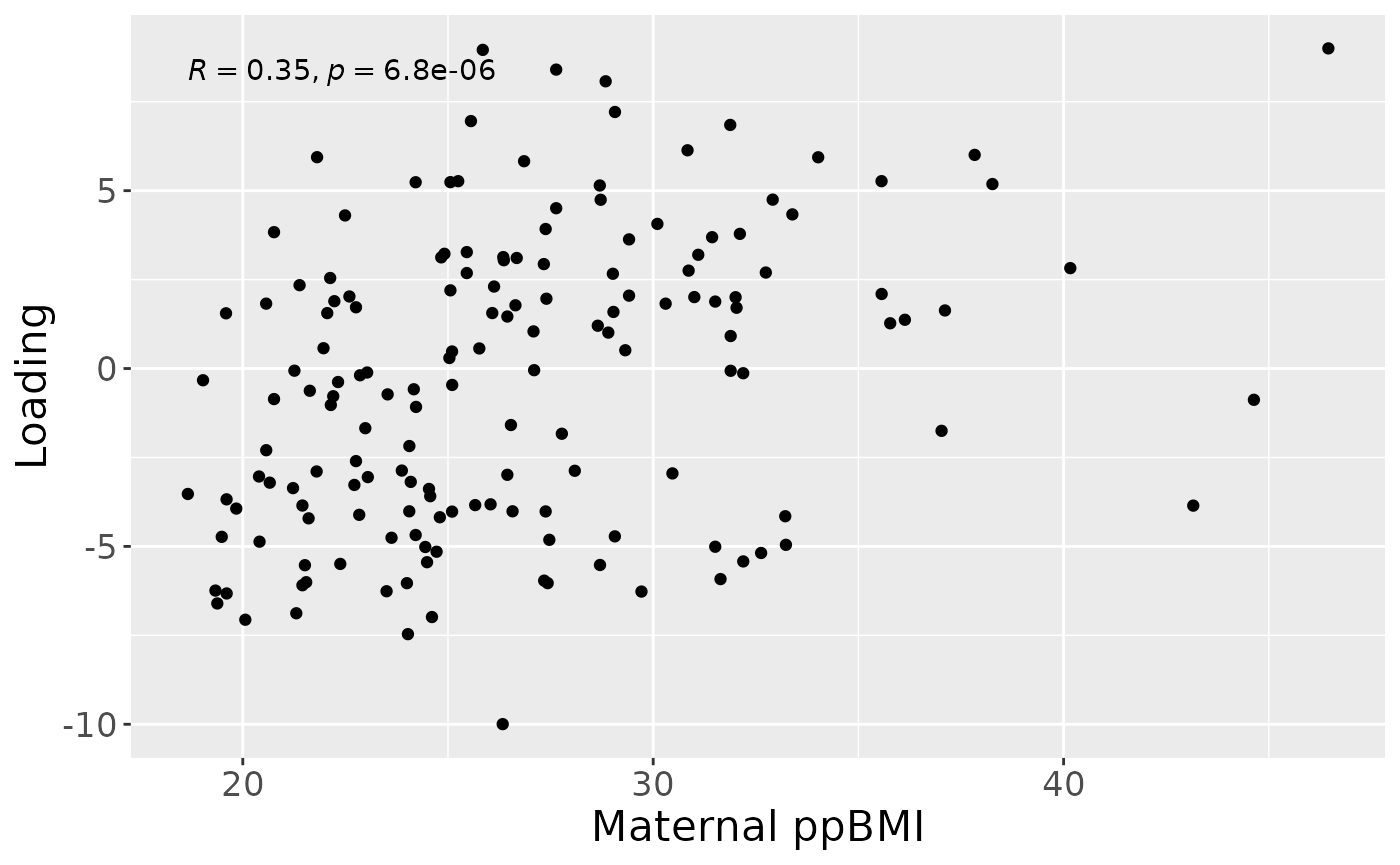
b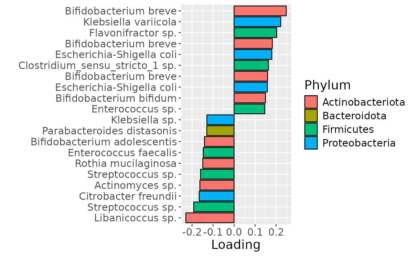
c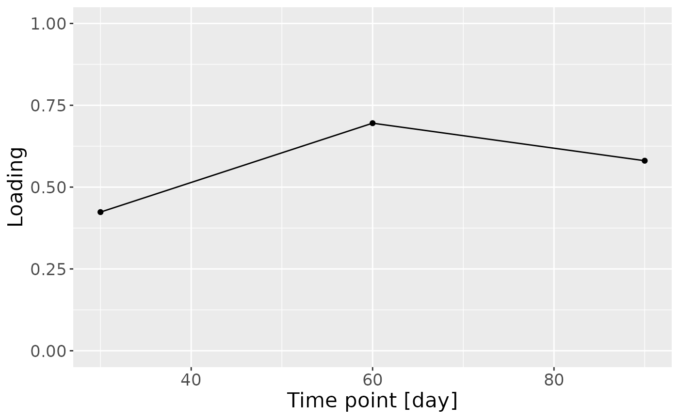
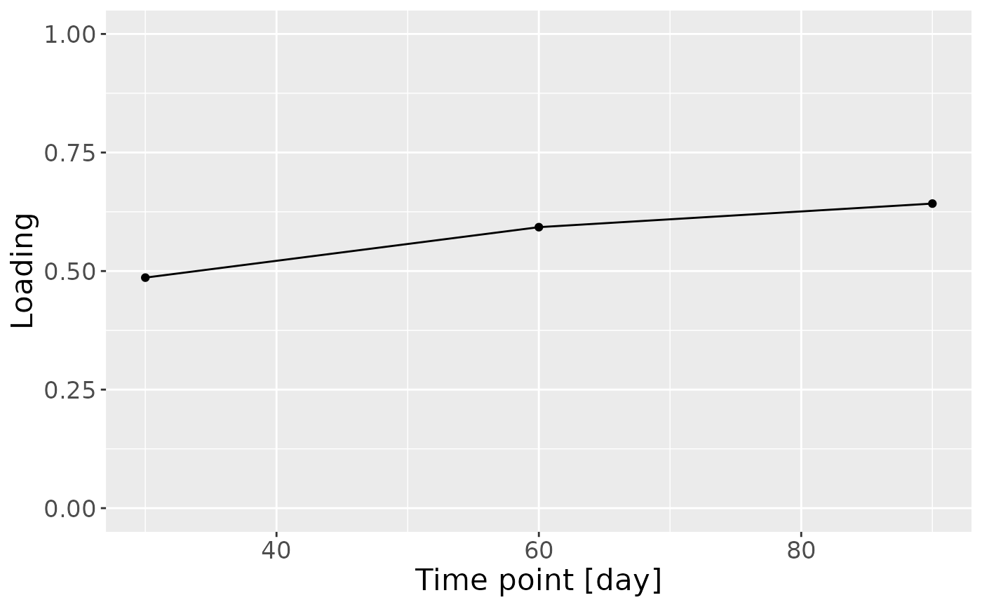
Positively loaded microbiota including Bifidobacterium breve, Bifidobacterium bifidum, Enterococcus sp., Escherichia coli, Clostridium} sp., and Staphylococcus epidermidis were enriched in infants of high ppBMI mothers and depleted in infants of low ppBMI mothers. Conversely, negatively loaded microbiota including Libanicoccus, Streptococcus, Actinomyces, and Klebsiella sp., as well as Citrobacter freundii, Rothia mucilaginosa, Enterococcus faecalis, Bifidobacterium adolescentis, and Parabacteroides distasonis were enriched in infants of low ppBMI mothers and depleted in infants of high ppBMI mothers. The time mode loadings indicate that ppBMI-associated inter-subject differences peaked at day 60.
HM microbiome
NPLS was next applied to supervise the decomposition using maternal pre-pregnancy BMI (ppBMI) as dependent variable (y). The model selection procedure revealed that a one-component model corresponded to the RMSECV minimum, explaining 5.4% of the variation in X, and 11.2% of the variation in y. The commented code below performs the procedure, and is not rerun here due to computational limitations.
# CV_milk = NPLStoolbox::ncrossreg(processedMilk$data, Ynorm_milk)
# a=CV_milk$varExp %>% pivot_longer(-numComponents) %>% ggplot(aes(x=as.factor(numComponents),y=value,col=as.factor(name),group=as.factor(name))) + geom_line() + geom_point() + xlab("Number of components") + ylab("Variance explained (%)") + theme(legend.position="none")
# b=CV_milk$RMSE %>% ggplot(aes(x=numComponents,y=RMSE)) + geom_line() + geom_point() + xlab("Number of components") + ylab("RMSECV")
# ggarrange(a,b) # 1 or 2 comps
# NPLS_milk = NPLStoolbox::triPLS1(processedMilk$data, Ynorm_milk, 1)
NPLS_milk = readRDS("./MAINHEALTH/20250702_NPLS_milk_bmi.RDS")

NPLS_milk$varExpX
#> [1] 5.310528
NPLS_milk$varExpY
#> [1] 11.21613
As expected, MLR analysis revealed that the model captured variation exclusively associated with maternal ppBMI.
testMetadata(NPLS_milk, 1, processedMilk)
#>        Term    Estimate                                       CI      P_value
#> 1       BMI   5.2632203 0.0028082806290875 – 0.00771815987488316 4.271728e-05
#> 2 C.section  22.5298730 -0.0223837277098485 – 0.0674434737293296 3.227116e-01
#> 3  Secretor  10.1431497  -0.0208977465387988 – 0.041184045914344 5.189801e-01
#> 4     Lewis -25.4005435  -0.113265523144618 – 0.0624644361527853 5.682343e-01
#> 5    whz.6m  -0.5937088  -0.012348966843658 – 0.0111615493028556 9.205334e-01
#>       P_adjust
#> 1 0.0002135864
#> 2 0.7102929209
#> 3 0.7102929209
#> 4 0.7102929209
#> 5 0.9205334443
# subject mode
a = processedMilk$mode1 %>%
  mutate(comp1 = NPLS_milk$Fac[[1]][,1]) %>%
  ggplot(aes(x=BMI,y=comp1)) +
  geom_point() +
  stat_cor() +
  xlab("Maternal ppBMI") +
  ylab("Loading") +
  theme(text=element_text(size=16))

# feature mode
topIndices = processedMilk$mode2 %>% mutate(index=1:nrow(.), Comp = NPLS_milk$Fac[[2]][,1]) %>% arrange(desc(Comp)) %>% head() %>% select(index) %>% pull()
bottomIndices = processedMilk$mode2 %>% mutate(index=1:nrow(.), Comp = NPLS_milk$Fac[[2]][,1]) %>% arrange(desc(Comp)) %>% tail() %>% select(index) %>% pull()

Xhat = parafac4microbiome::reinflateTensor(NPLS_milk$Fac[[1]][,1], NPLS_milk$Fac[[2]][,1], NPLS_milk$Fac[[3]][,1])

print("Positive loadings:")
#> [1] "Positive loadings:"
print(cor(Xhat[,topIndices[1],1], processedMilk$mode1$BMI)) # flip
#> [1] -0.3351345
print("Negative loadings:")
#> [1] "Negative loadings:"
print(cor(Xhat[,bottomIndices[1],1], processedMilk$mode1$BMI))
#> [1] 0.3351345

df = processedMilk$mode2 %>%
  mutate(Component_1 = -1*NPLS_milk$Fac[[2]][,1]) %>%
  arrange(Component_1) %>%
  mutate(index=1:nrow(.)) %>%
  mutate(Genus = gsub("g__", "", V7), Species = gsub("s__", "", V8)) %>%
  mutate(Species = str_split_fixed(Species, "_", 2)[,2]) %>%
  mutate(dplyr::across(.cols = Species, .fns = ~ dplyr::if_else(stringr::str_detect(.x, "sp."), "", .x))) %>%
  mutate(dplyr::across(.cols = Species, .fns = ~ dplyr::if_else(stringr::str_detect(.x, "organism"), "", .x))) %>%
  mutate(dplyr::across(.cols = Species, .fns = ~ dplyr::if_else(stringr::str_detect(.x, "bacterium"), "", .x))) %>%
  filter(index %in% c(1:10, 106:115))

df[df$Genus == "" & df$Species == "", "Species"] = "Unknown"
df[df$Species == "", "Species"] = "sp."
df$name = paste0(df$Genus, " ", df$Species)

b = df %>% ggplot(aes(x=Component_1,y=as.factor(index),fill=as.factor(V3))) +
  geom_bar(stat="identity", col="black") +
  xlab("Loading") +
  ylab("") +
  scale_y_discrete(labels=df$name) +
  scale_fill_manual(name="Phylum", values=hue_pal()(5)[-5], labels=c("Actinobacteriota", "Bacteroidota", "Firmicutes", "Proteobacteria")) +
  theme(text=element_text(size=16))

# time mode
c = NPLS_milk$Fac[[3]][,1] %>%
  as_tibble() %>%
  mutate(value=-1*value) %>%
  ggplot(aes(x=c(0,30,60,90),y=value)) +
  geom_line() +
  geom_point() +
  xlab("Time point [day]") +
  ylab("Loading") +
  ylim(0,1) +
  theme(text=element_text(size=16))

a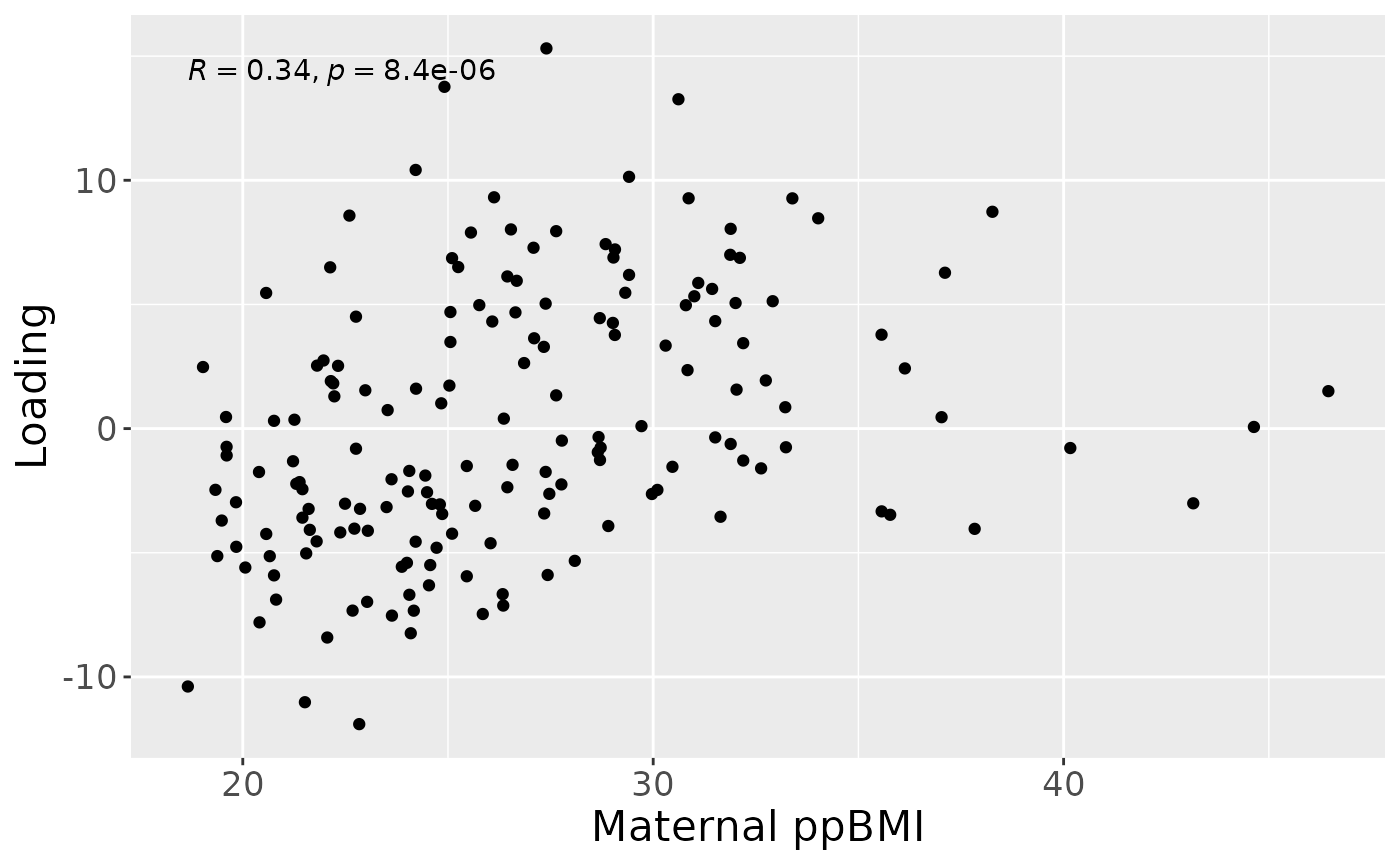
b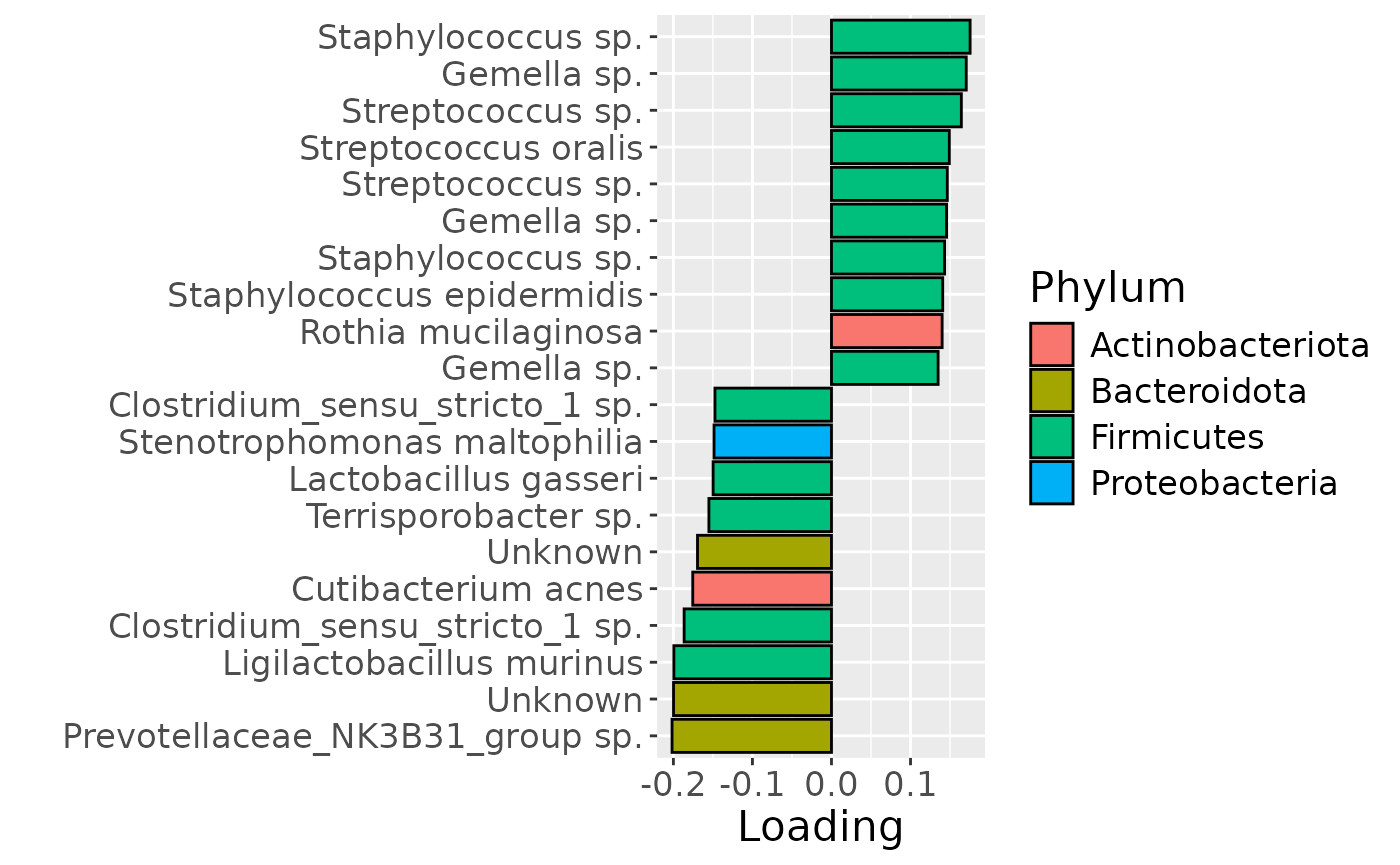
c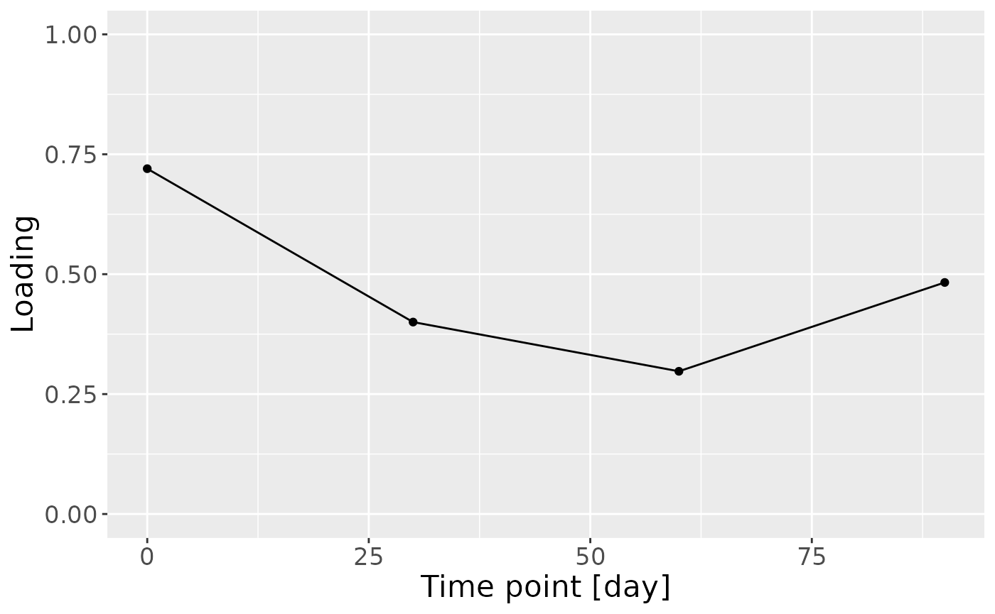
Positively loaded microbiota including Gemella, Streptococcus and Staphylococcus spp. were enriched in high ppBMI mothers and depleted in low ppBMI mothers. Conversely, negatively loaded microbiota including Ligilactobacillus murinus, Clostridium sensu stricto spp., Cutibacterium acnes, Terrisporobacter sp., Lactobacillus gasseri, and Stenotrophomonas maltophilia were enriched in low ppBMI mothers and depleted in high ppBMI mothers. The time mode loadings indicated that inter-subject differences due to maternal ppBMI were largest at day 0 and declined over time.
HM metabolome
NPLS was next applied to supervise the decomposition using maternal pre-pregnancy BMI (ppBMI) as dependent variable (y). While the model selection procedure revealed that a two-component NPLS model corresponded to the RMSECV minimum, we found that the extra component did not help in the prediction of y, nor was it biologically interpretable. Hence, a one-component NPLS model was fitted, explaining 3.1% of the variation in X, and 31.0% of the variation in y. The commented code below performs the procedure, and is not rerun here due to computational limitations.
# CV_milkMetab = NPLStoolbox::ncrossreg(processedMilkMetab$data, Ynorm_milkMetab)
# a=CV_milkMetab$varExp %>% pivot_longer(-numComponents) %>% ggplot(aes(x=as.factor(numComponents),y=value,col=as.factor(name),group=as.factor(name))) + geom_line() + geom_point() + xlab("Number of components") + ylab("Variance explained (%)") + theme(legend.position="none")
# b=CV_milkMetab$RMSE %>% ggplot(aes(x=numComponents,y=RMSE)) + geom_line() + geom_point() + xlab("Number of components") + ylab("RMSECV")
# ggarrange(a,b) # 1 comp
# NPLS_milkMetab = NPLStoolbox::triPLS1(processedMilkMetab$data, Ynorm_milkMetab, 2)
NPLS_milkMetab = readRDS("./MAINHEALTH/20250702_NPLS_milkMetab_bmi.RDS")

NPLS_milkMetab$varExpX
#> [1] 3.057919
NPLS_milkMetab$varExpY
#> [1] 31.03798
However, MLR analysis revealed that the model captured variation associated with a mixture of maternal ppBMI, maternal secretor status, and infant growth at 6 months.
testMetadata(NPLS_milkMetab, 1, processedMilkMetab)
#>        Term   Estimate                                         CI      P_value
#> 1       BMI   8.436042   0.00639137955287423 – 0.0104807043090265 2.963990e-13
#> 2 C.section  12.030701   -0.0252983772275604 – 0.0493597786809759 5.247398e-01
#> 3  Secretor  30.260127    0.00416557076519333 – 0.056354683431391 2.339660e-02
#> 4     Lewis -80.278456    -0.16922492265323 – 0.00866801160802368 7.648230e-02
#> 5    whz.6m -12.918737 -0.0226848901579012 – -0.00315258357667813 9.937333e-03
#>       P_adjust
#> 1 1.481995e-12
#> 2 5.247398e-01
#> 3 3.899434e-02
#> 4 9.560288e-02
#> 5 2.484333e-02
# subject mode
a = processedMilkMetab$mode1 %>%
  mutate(comp1 = NPLS_milkMetab$Fac[[1]][,1]) %>%
  ggplot(aes(x=BMI,y=comp1)) +
  geom_point() +
  stat_cor() +
  xlab("Maternal ppBMI") +
  ylab("Loading") +
  theme(text=element_text(size=16))

# feature mode
topIndices = processedMilkMetab$mode2 %>% mutate(index=1:nrow(.), Comp = NPLS_milkMetab$Fac[[2]][,1]) %>% arrange(desc(Comp)) %>% head() %>% select(index) %>% pull()
bottomIndices = processedMilkMetab$mode2 %>% mutate(index=1:nrow(.), Comp = NPLS_milkMetab$Fac[[2]][,1]) %>% arrange(desc(Comp)) %>% tail() %>% select(index) %>% pull()

Xhat = parafac4microbiome::reinflateTensor(NPLS_milkMetab$Fac[[1]][,1], NPLS_milkMetab$Fac[[2]][,1], NPLS_milkMetab$Fac[[3]][,1])

print("Positive loadings:")
#> [1] "Positive loadings:"
print(cor(Xhat[,topIndices[1],1], processedMilkMetab$mode1$BMI))
#> [1] 0.5572628
print("Negative loadings:")
#> [1] "Negative loadings:"
print(cor(Xhat[,bottomIndices[1],1], processedMilkMetab$mode1$BMI))
#> [1] -0.5572628

temp = processedMilkMetab$mode2 %>% mutate(Component_1 = NPLS_milkMetab$Fac[[2]][,1]) %>% arrange(Component_1) %>% mutate(index=1:nrow(.)) %>% filter(index %in% c(1:10, 61:70))

b=temp %>%
  ggplot(aes(x=Component_1,y=as.factor(index),fill=as.factor(Class),pattern=as.factor(Class))) +
  geom_bar_pattern(stat="identity",
                   colour="black",
                   pattern="stripe",
                   pattern_fill="black",
                   pattern_density=0.2,
                   pattern_spacing=0.05,
                   pattern_angle=45,
                   pattern_size=0.2) +
  scale_y_discrete(label=temp$Metabolite) +
  xlab("Loading") +
  ylab("") +
  scale_fill_manual(name="Class", values=hue_pal()(7)[-5], labels=c("Amino acids and derivatives", "Energy related", "Fatty acids and derivatives", "Food derived", "Oligosaccharides", "Sugars")) +
  theme(text=element_text(size=16), legend.position="none")

# time mode
c = NPLS_milkMetab$Fac[[3]][,1] %>%
  as_tibble() %>%
  mutate(value=value) %>%
  ggplot(aes(x=c(0,30,60,90),y=value)) +
  geom_line() +
  geom_point() +
  xlab("Time point [day]") +
  ylab("Loading") +
  ylim(0,1) +
  theme(text=element_text(size=16))

a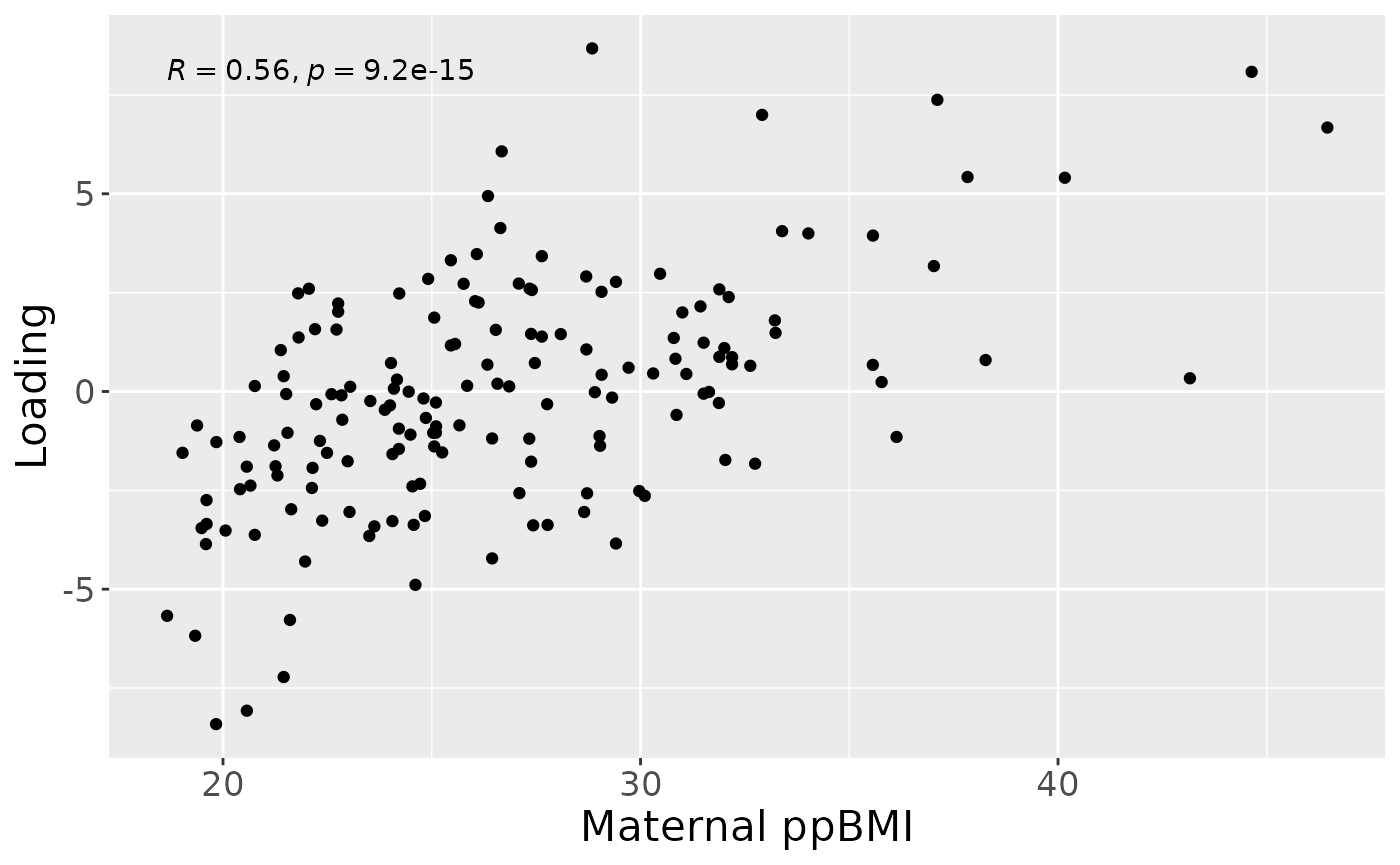
b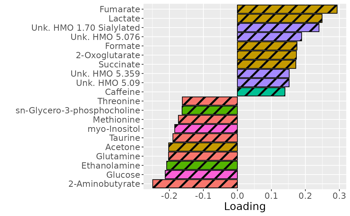
c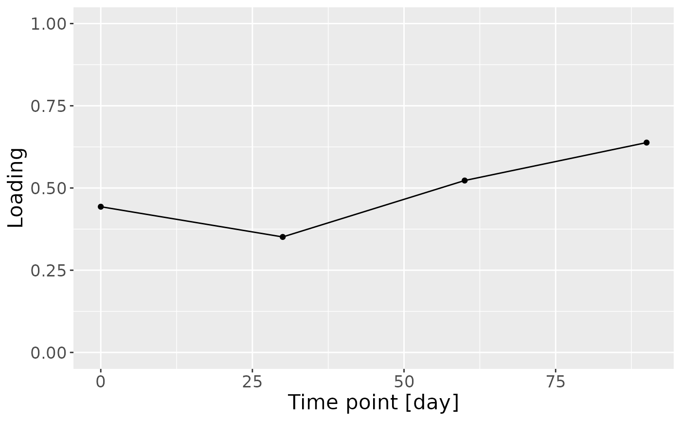
Infant weight-over-height z-score at six months
Processing
# Faeces
newFaeces = NPLStoolbox::Jakobsen2025$faeces

mask1 = newFaeces$mode1$subject %in% (NPLStoolbox::Jakobsen2025$faeces$mode1 %>% filter(!is.na(whz.6m)) %>% select(subject) %>% pull())
mask2 = newFaeces$mode1$subject != "322"
mask = mask1 & mask2
newFaeces$data = newFaeces$data[mask,,]
newFaeces$mode1 = newFaeces$mode1[mask,]
processedFaeces = parafac4microbiome::processDataCube(newFaeces, sparsityThreshold = 0.75, centerMode=1, scaleMode=2) # was 0.75

# Milk
newMilk = NPLStoolbox::Jakobsen2025$milkMicrobiome

mask = newMilk$mode1$subject %in% (NPLStoolbox::Jakobsen2025$milkMicrobiome$mode1 %>% filter(!is.na(whz.6m)) %>% select(subject) %>% pull())
newMilk$data = newMilk$data[mask,,]
newMilk$mode1 = newMilk$mode1[mask,]
processedMilk = parafac4microbiome::processDataCube(newMilk, sparsityThreshold=0.85, centerMode=1, scaleMode=2) # was 0.85

# Milk metab
newMilkMetab = NPLStoolbox::Jakobsen2025$milkMetabolomics

mask = newMilkMetab$mode1$subject %in% (NPLStoolbox::Jakobsen2025$milkMetabolomics$mode1 %>% filter(!is.na(whz.6m)) %>% select(subject) %>% pull())
newMilkMetab$data = newMilkMetab$data[mask,,-1]
newMilkMetab$mode1 = newMilkMetab$mode1[mask,]
newMilkMetab$mode3 = newMilkMetab$mode3[-1,]
processedMilkMetab = parafac4microbiome::processDataCube(newMilkMetab, CLR=FALSE, centerMode=1, scaleMode=2)Infant faecal microbiome
Subsequently, NPLS was applied to supervise the decomposition using the infant growth weight-for-height at six months (WHZ) as dependent variable (y). The model selection procedure revealed that a one-component NPLS model corresponded to the RMSECV minimum, explaining 2.6% of the variation in X, and 11.2% of the variation in y. The commented code below performs the procedure, and is not rerun here due to computational limitations.
# CV_faecal = NPLStoolbox::ncrossreg(processedFaeces$data, Ynorm_faecal)
# a=CV_faecal$varExp %>% pivot_longer(-numComponents) %>% ggplot(aes(x=as.factor(numComponents),y=value,col=as.factor(name),group=as.factor(name))) + geom_line() + geom_point() + xlab("Number of components") + ylab("Variance explained (%)") + theme(legend.position="none")
# b=CV_faecal$RMSE %>% ggplot(aes(x=numComponents,y=RMSE)) + geom_line() + geom_point() + xlab("Number of components") + ylab("RMSECV")
# ggarrange(a,b) # 1 comp
# NPLS_faecal = NPLStoolbox::triPLS1(processedFaeces$data, Ynorm_faecal, 1)
NPLS_faecal = readRDS("./MAINHEALTH/20250702_NPLS_faecal_whz.RDS")

NPLS_faecal$varExpX
#> [1] 2.586198
NPLS_faecal$varExpY
#> [1] 11.22538
As expected, MLR analysis revealed that the model captured variation exclusively associated with maternal ppBMI.
testMetadata(NPLS_faecal, 1, processedFaeces)
#>        Term   Estimate                                          CI      P_value
#> 1       BMI   2.110906 -0.000563660471044009 – 0.00478547212944011 0.1208012322
#> 2 C.section  48.317474  -0.000583193126835087 – 0.0972181419517821 0.0527523625
#> 3  Secretor  17.889671    -0.0159154384713816 – 0.0516947797774786 0.2969361598
#> 4     Lewis -83.311435     -0.178990514960686 – 0.0123676446394298 0.0873024247
#> 5    whz.6m  23.212088     0.0104288246136979 – 0.0359953513693422 0.0004681401
#>    P_adjust
#> 1 0.1510015
#> 2 0.1318809
#> 3 0.2969362
#> 4 0.1455040
#> 5 0.0023407
# subject mode
a = processedFaeces$mode1 %>%
  mutate(comp1 = NPLS_faecal$Fac[[1]][,1]) %>%
  ggplot(aes(x=whz.6m,y=comp1)) +
  geom_point() +
  stat_cor() +
  xlab("Infant 6-month WHZ") +
  ylab("Loading") +
  theme(text=element_text(size=16))

# feature mode
topIndices = processedFaeces$mode2 %>% mutate(index=1:nrow(.), Comp = NPLS_faecal$Fac[[2]][,1]) %>% arrange(desc(Comp)) %>% head() %>% select(index) %>% pull()
bottomIndices = processedFaeces$mode2 %>% mutate(index=1:nrow(.), Comp = NPLS_faecal$Fac[[2]][,1]) %>% arrange(desc(Comp)) %>% tail() %>% select(index) %>% pull()

Xhat = parafac4microbiome::reinflateTensor(NPLS_faecal$Fac[[1]][,1], NPLS_faecal$Fac[[2]][,1], NPLS_faecal$Fac[[3]][,1])

print("Positive loadings:")
#> [1] "Positive loadings:"
print(cor(Xhat[,topIndices[1],1], processedFaeces$mode1$whz.6m))
#> [1] -0.3351143
print("Negative loadings:")
#> [1] "Negative loadings:"
print(cor(Xhat[,bottomIndices[1],1], processedFaeces$mode1$whz.6m))
#> [1] 0.3351143

df = processedFaeces$mode2 %>%
  mutate(Component_1 = -1*NPLS_faecal$Fac[[2]][,1]) %>%
  arrange(Component_1) %>%
  mutate(index=1:nrow(.)) %>%
  mutate(Genus = gsub("g__", "", V7), Species = gsub("s__", "", V8)) %>%
  mutate(Species = str_split_fixed(Species, "_", 2)[,2]) %>%
  mutate(dplyr::across(.cols = Species, .fns = ~ dplyr::if_else(stringr::str_detect(.x, "sp."), "", .x))) %>%
  mutate(dplyr::across(.cols = Species, .fns = ~ dplyr::if_else(stringr::str_detect(.x, "organism"), "", .x))) %>%
  mutate(dplyr::across(.cols = Species, .fns = ~ dplyr::if_else(stringr::str_detect(.x, "bacterium"), "", .x))) %>%
  filter(index %in% c(1:10, 84:93))

df[df$Genus == "" & df$Species == "", "Species"] = "Unknown"
df[df$Species == "", "Species"] = "sp."
df$name = paste0(df$Genus, " ", df$Species)

b = df %>% ggplot(aes(x=Component_1,y=as.factor(index),fill=as.factor(V3))) +
  geom_bar(stat="identity", col="black") +
  xlab("Loading") +
  ylab("") +
  scale_y_discrete(labels=df$name) +
  scale_fill_manual(name="Phylum", values=hue_pal()(5)[-5], labels=c("Actinobacteriota", "Bacteroidota", "Firmicutes", "Proteobacteria")) +
  theme(text=element_text(size=16))

# time mode
c = NPLS_faecal$Fac[[3]][,1] %>%
  as_tibble() %>%
  mutate(value=-1*value) %>%
  ggplot(aes(x=c(30,60,90),y=value)) +
  geom_line() +
  geom_point() +
  xlab("Time point [day]") +
  ylab("Loading") +
  ylim(0,1) +
  theme(text=element_text(size=16))

a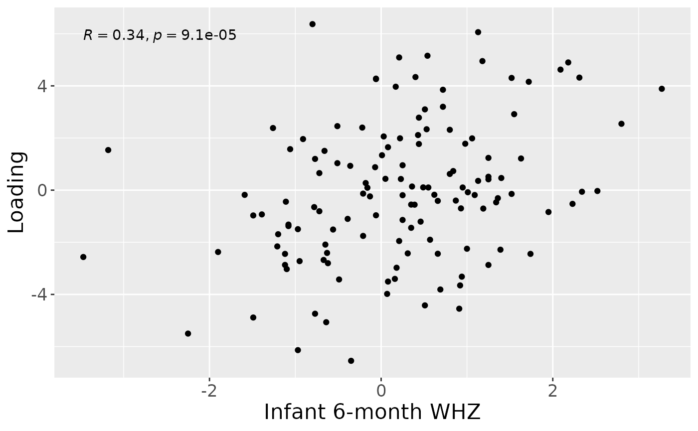
b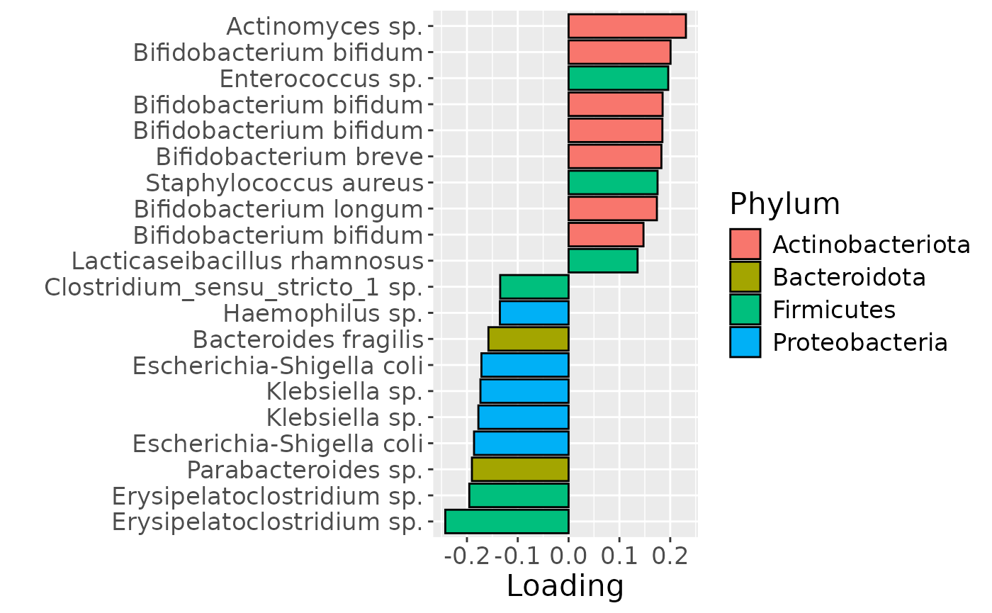
c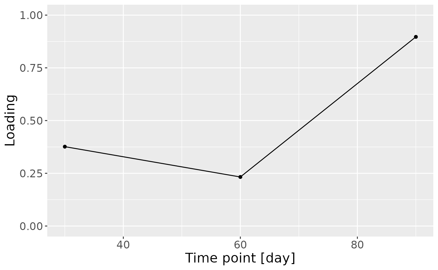
Positively loaded microbiota included many Actinobacteriota such as Actinomyces sp., Bifidobacterium bifidum, Bifidobacterium breve, and Bifidobacterium longum}, as well as Enterococcus sp., Straphylococcus aureus, and Lacticaseibacillus rhamnosus, which were enriched in high-growth infants and depleted in low-growth infants. Conversely, negatively loaded microbiota included many Proteobacteria such as Escherichia-Shigella coli, Klepsiella spp., and Haemophilus sp., as well as Erysipelatoclostridium spp., Parabacteroides sp., Bacteroides fragilis, and Clostridium sensu stricto sp., which were enriched in low-growth infants and depleted in high-growth infants. The time mode loadings indicated that these inter-subject differences were maximal at day 90.
HM microbiome
Subsequently, NPLS was applied to supervise the decomposition using the infant growth weight-for-height at six months (WHZ) as dependent variable (y). While the model selection procedure revealed that a two-component model corresponded to the RMSECV minimum, we found that the extra component did not help in the prediction of y, nor was it biologically interpretable. Hence, a one-component NPLS model was fitted, explaining 1.6% of the variation in X, and 9.7% of the variation in y. The commented code below performs the procedure, and is not rerun here due to computational limitations.
# CV_milk = NPLStoolbox::ncrossreg(processedMilk$data, Ynorm_milk)
# a=CV_milk$varExp %>% pivot_longer(-numComponents) %>% ggplot(aes(x=as.factor(numComponents),y=value,col=as.factor(name),group=as.factor(name))) + geom_line() + geom_point() + xlab("Number of components") + ylab("Variance explained (%)") + theme(legend.position="none")
# b=CV_milk$RMSE %>% ggplot(aes(x=numComponents,y=RMSE)) + geom_line() + geom_point() + xlab("Number of components") + ylab("RMSECV")
# ggarrange(a,b) # 1 or 2 comps
# NPLS_milk = NPLStoolbox::triPLS1(processedMilk$data, Ynorm_milk, 1)
NPLS_milk = readRDS("./MAINHEALTH/20250702_NPLS_milk_whz.RDS")

NPLS_milk$varExpX
#> [1] 1.583301
NPLS_milk$varExpY
#> [1] 9.744233
However, MLR analysis revealed that the model captured variation associated with a mixture of infant WHZ and maternal ppBMI.
testMetadata(NPLS_milk, 1, processedMilk)
#>        Term  Estimate                                         CI      P_value
#> 1       BMI  3.619784 0.000919112513437887 – 0.00632045481617513 0.0090248586
#> 2 C.section 28.892024   -0.0205172827975998 – 0.0783013314250206 0.2493411802
#> 3  Secretor  7.069697   -0.0270782924260968 – 0.0412176869697414 0.6826797911
#> 4     Lewis -6.834201    -0.103494181064122 – 0.0898257796709901 0.8889328165
#> 5    whz.6m 23.511923    0.0105800019938657 – 0.0364438448837068 0.0004607509
#>      P_adjust
#> 1 0.022562147
#> 2 0.415568634
#> 3 0.853349739
#> 4 0.888932817
#> 5 0.002303755
# subject mode
a = processedMilk$mode1 %>%
  mutate(comp1 = NPLS_milk$Fac[[1]][,1]) %>%
  ggplot(aes(x=whz.6m,y=comp1)) +
  geom_point() +
  stat_cor() +
  xlab("Maternal ppBMI") +
  ylab("Loading") +
  theme(text=element_text(size=16))

# feature mode
topIndices = processedMilk$mode2 %>% mutate(index=1:nrow(.), Comp = NPLS_milk$Fac[[2]][,1]) %>% arrange(desc(Comp)) %>% head() %>% select(index) %>% pull()
bottomIndices = processedMilk$mode2 %>% mutate(index=1:nrow(.), Comp = NPLS_milk$Fac[[2]][,1]) %>% arrange(desc(Comp)) %>% tail() %>% select(index) %>% pull()

Xhat = parafac4microbiome::reinflateTensor(NPLS_milk$Fac[[1]][,1], NPLS_milk$Fac[[2]][,1], NPLS_milk$Fac[[3]][,1])

print("Positive loadings:")
#> [1] "Positive loadings:"
print(cor(Xhat[,topIndices[1],1], processedMilk$mode1$whz.6m)) # flip
#> [1] 0.312612
print("Negative loadings:")
#> [1] "Negative loadings:"
print(cor(Xhat[,bottomIndices[1],1], processedMilk$mode1$whz.6m))
#> [1] -0.312612

df = processedMilk$mode2 %>%
  mutate(Component_1 = -1*NPLS_milk$Fac[[2]][,1]) %>%
  arrange(Component_1) %>%
  mutate(index=1:nrow(.)) %>%
  mutate(Genus = gsub("g__", "", V7), Species = gsub("s__", "", V8)) %>%
  mutate(Species = str_split_fixed(Species, "_", 2)[,2]) %>%
  mutate(dplyr::across(.cols = Species, .fns = ~ dplyr::if_else(stringr::str_detect(.x, "sp."), "", .x))) %>%
  mutate(dplyr::across(.cols = Species, .fns = ~ dplyr::if_else(stringr::str_detect(.x, "organism"), "", .x))) %>%
  mutate(dplyr::across(.cols = Species, .fns = ~ dplyr::if_else(stringr::str_detect(.x, "bacterium"), "", .x))) %>%
  filter(index %in% c(1:10, 106:115))

df[df$Genus == "" & df$Species == "", "Species"] = "Unknown"
df[df$Species == "", "Species"] = "sp."
df$name = paste0(df$Genus, " ", df$Species)

b = df %>% ggplot(aes(x=Component_1,y=as.factor(index),fill=as.factor(V3))) +
  geom_bar(stat="identity", col="black") +
  xlab("Loading") +
  ylab("") +
  scale_y_discrete(labels=df$name) +
  theme(text=element_text(size=16))

# time mode
c = NPLS_milk$Fac[[3]][,1] %>%
  as_tibble() %>%
  mutate(value=-1*value) %>%
  ggplot(aes(x=c(0,30,60,90),y=value)) +
  geom_line() +
  geom_point() +
  xlab("Time point [day]") +
  ylab("Loading") +
  ylim(0,1) +
  theme(text=element_text(size=16))

a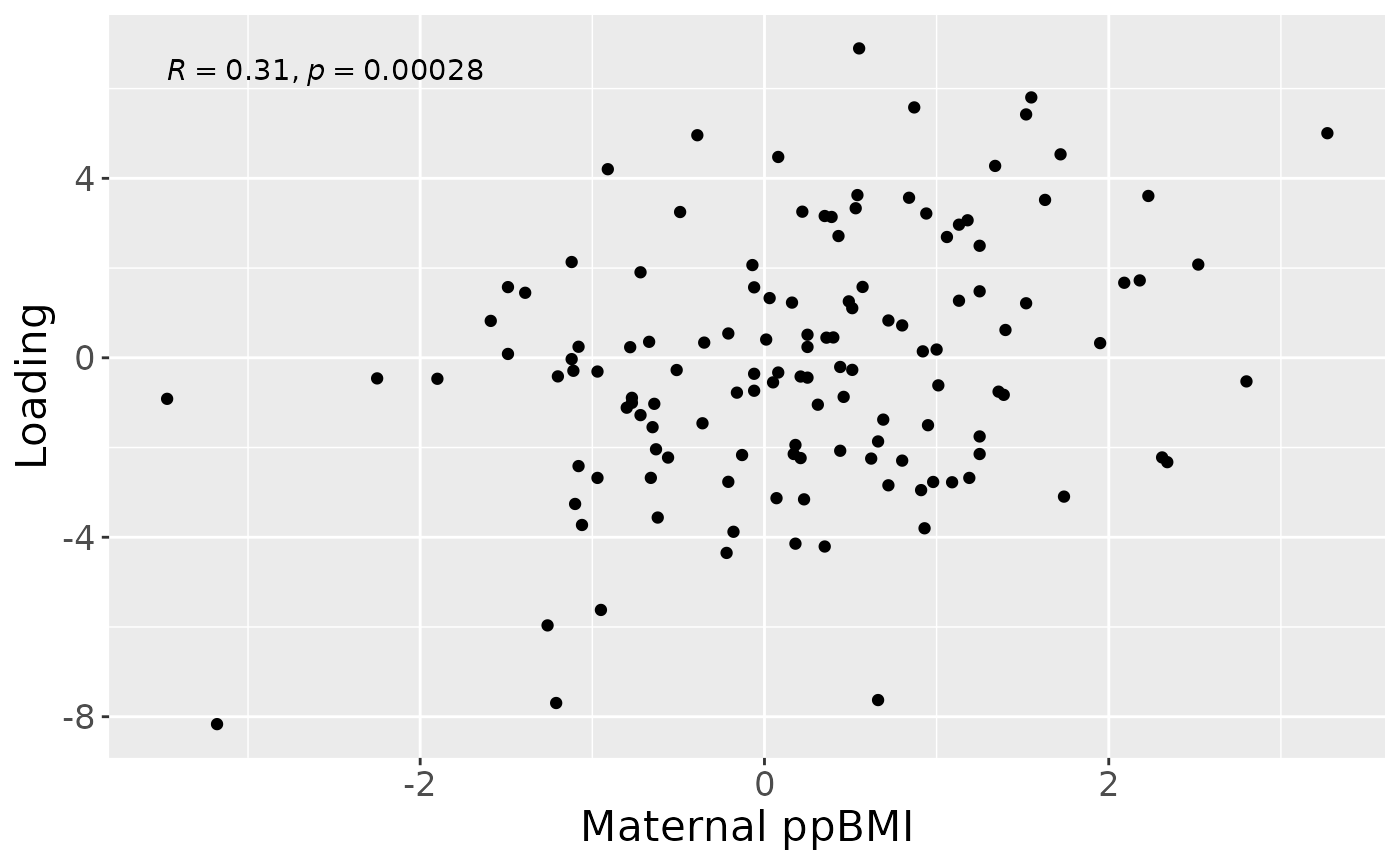
b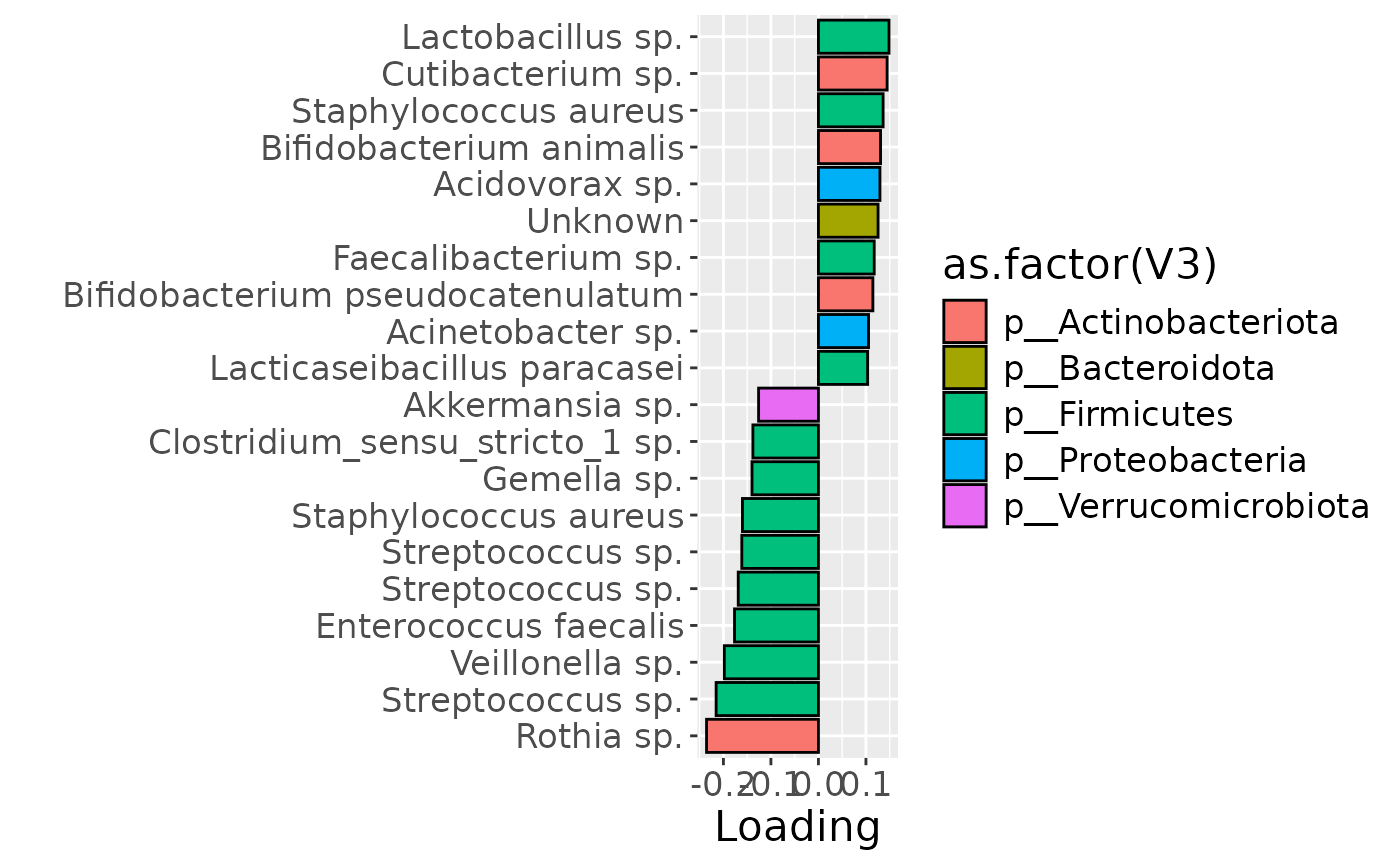
c
#> Warning: Removed 4 rows containing missing values or values outside the scale range
#> (`geom_line()`).
#> Warning: Removed 4 rows containing missing values or values outside the scale range
#> (`geom_point()`).
HM metabolome
Subsequently, NPLS was applied to supervise the decomposition using the infant growth weight-for-height at six months (WHZ) as dependent variable (y). The model selection procedure revealed that a one-component NPLS model corresponded to the RMSECV minimum, explaining 4.2% of the variation in X, and 15.8% of the variation in y. The commented code below performs the procedure, and is not rerun here due to computational limitations.
# CV_milkMetab = NPLStoolbox::ncrossreg(processedMilkMetab$data, Ynorm_milkMetab)
# a=CV_milkMetab$varExp %>% pivot_longer(-numComponents) %>% ggplot(aes(x=as.factor(numComponents),y=value,col=as.factor(name),group=as.factor(name))) + geom_line() + geom_point() + xlab("Number of components") + ylab("Variance explained (%)") + theme(legend.position="none")
# b=CV_milkMetab$RMSE %>% ggplot(aes(x=numComponents,y=RMSE)) + geom_line() + geom_point() + xlab("Number of components") + ylab("RMSECV")
# ggarrange(a,b) # 1 comp
# NPLS_milkMetab = NPLStoolbox::triPLS1(processedMilkMetab$data, Ynorm_milkMetab, 2)
NPLS_milkMetab = readRDS("./MAINHEALTH/20250702_NPLS_milkMetab_whz.RDS")

NPLS_milkMetab$varExpX
#> [1] 4.212077
NPLS_milkMetab$varExpY
#> [1] 15.79571
However, MLR analysis revealed that the model captured variation associated with a mixture of infant growth, but also maternal ppBMI and maternal secretor status.
testMetadata(NPLS_milkMetab, 1, processedMilkMetab)
#>        Term   Estimate                                        CI      P_value
#> 1       BMI  -4.201449 -0.0065484366313087 – -0.0018544615122335 5.571588e-04
#> 2 C.section -13.368907  -0.0562174881702821 – 0.0294796738718076 5.380324e-01
#> 3  Secretor -80.629893  -0.110582808524329 – -0.0506769778677665 4.475097e-07
#> 4     Lewis  39.067983    -0.0630301697222898 – 0.14116613579865 4.502868e-01
#> 5    whz.6m  30.446281   0.0192360974045573 – 0.0416564642322284 3.612822e-07
#>       P_adjust
#> 1 9.285980e-04
#> 2 5.380324e-01
#> 3 1.118774e-06
#> 4 5.380324e-01
#> 5 1.118774e-06
# subject mode
a = processedMilkMetab$mode1 %>%
  mutate(comp1 = NPLS_milkMetab$Fac[[1]][,1]) %>%
  ggplot(aes(x=whz.6m,y=comp1)) +
  geom_point() +
  stat_cor() +
  xlab("Maternal ppBMI") +
  ylab("Loading") +
  theme(text=element_text(size=16))

# feature mode
topIndices = processedMilkMetab$mode2 %>% mutate(index=1:nrow(.), Comp = NPLS_milkMetab$Fac[[2]][,1]) %>% arrange(desc(Comp)) %>% head() %>% select(index) %>% pull()
bottomIndices = processedMilkMetab$mode2 %>% mutate(index=1:nrow(.), Comp = NPLS_milkMetab$Fac[[2]][,1]) %>% arrange(desc(Comp)) %>% tail() %>% select(index) %>% pull()

Xhat = parafac4microbiome::reinflateTensor(NPLS_milkMetab$Fac[[1]][,1], NPLS_milkMetab$Fac[[2]][,1], NPLS_milkMetab$Fac[[3]][,1])

print("Positive loadings:")
#> [1] "Positive loadings:"
print(cor(Xhat[,topIndices[1],1], processedMilkMetab$mode1$whz.6m))
#> [1] -0.3974434
print("Negative loadings:")
#> [1] "Negative loadings:"
print(cor(Xhat[,bottomIndices[1],1], processedMilkMetab$mode1$whz.6m))
#> [1] 0.3974434

temp = processedMilkMetab$mode2 %>% mutate(Component_1 = NPLS_milkMetab$Fac[[2]][,1]) %>% arrange(Component_1) %>% mutate(index=1:nrow(.)) %>% filter(index %in% c(1:10, 61:70))

b=temp %>%
  ggplot(aes(x=Component_1,y=as.factor(index),fill=as.factor(Class),pattern=as.factor(Class))) +
  geom_bar_pattern(stat="identity",
                   colour="black",
                   pattern="stripe",
                   pattern_fill="black",
                   pattern_density=0.2,
                   pattern_spacing=0.05,
                   pattern_angle=45,
                   pattern_size=0.2) +
  scale_y_discrete(label=temp$Metabolite) +
  xlab("Loading") +
  ylab("") +
  theme(text=element_text(size=16), legend.position="none")

# time mode
c = NPLS_milkMetab$Fac[[3]][,1] %>%
  as_tibble() %>%
  mutate(value=-1*value, timepoints = c(30,60,90)) %>%
  ggplot(aes(x=timepoints,y=value)) +
  geom_line() +
  geom_point() +
  xlab("Time point [day]") +
  ylab("Loading") +
  ylim(0,1) +
  theme(text=element_text(size=16))

a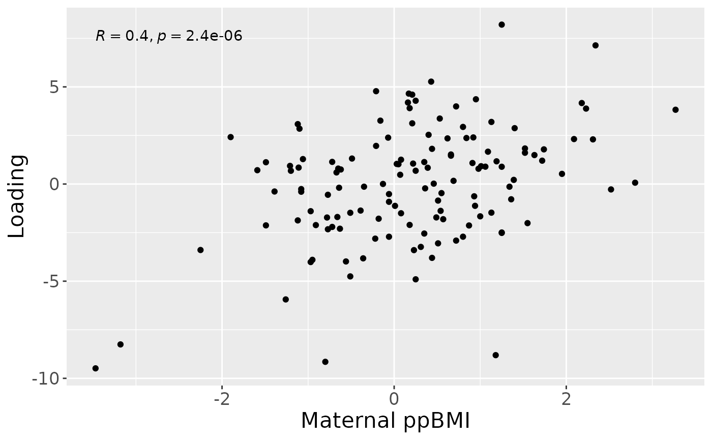
b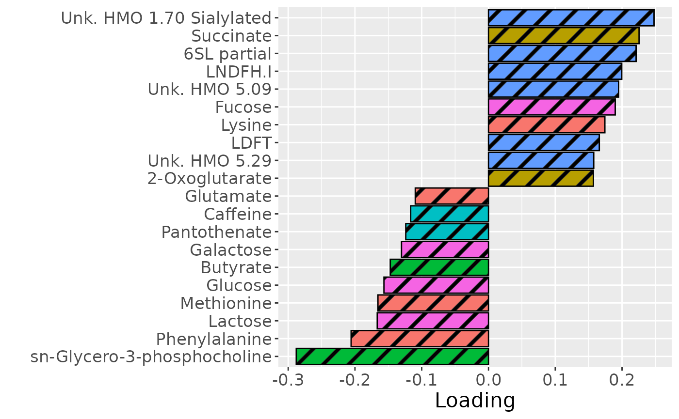
c